In addition to individual tangent vectors, MTEX allows defining vector fields on the rotation group via the SO3VectorField class. A vector field maps rotations to tangent vectors, i.e., when evaluated at a rotation \(R\), it returns a SO3TangentVector.
For background on the structure of the tangent space on SO(3) and the definition of @SO3TangentVectors in MTEX, see the documentation page SO(3) Tangent Space.
Vector fields in orientation space model orientation dependent spin as it occurs for instance in the Taylor or Sachs model. Another typical example are gradients of orientation distribution functions.
Lets consider the following ODF of a quartz specimen Then its gradient is computed by the command odf.grad
odf = SO3Fun.dubna;
G = odf.grad

% Evaluation of the Gradient in some rotations
rot = rotation.rand(3);
G.eval(rot)
G = SO3VectorFieldHarmonic (Quartz → y↑→x)
bandwidth: 48
tangent space: leftVector
ans = SO3TangentVector (y↑→x)
intern symmetries: Quartz → y↑→x
size: 3 x 1
TagentSpace: leftVector
x y z
-0.027 0.508 -0.0764
0.659 -0.375 0.825
-0.396 1.06 0.413Lets visualize the ODF together with its gradient in a sigma section plot
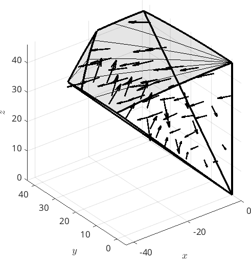
plot(odf,'sigma')
hold on
plot(G,'linewidth',1.5,'color','black','resolution',7.5*degree)
hold off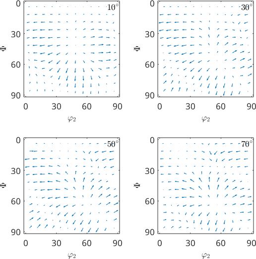
We observe how the gradients all points towards the closest local maximum. This is actually the foundation of the steepest descent algorithm used by MTEX in the commands max(odf) and calcComponents(odf)
Table of Contents
Representations of SO3VectorFields
Internally MTEX represents @SO3VectorFields in different ways:
|
a vector valued SO3FunHarmonic (3 components) |
|
|
a vector valued SO3FunRBF (3 components) |
|
|
explicitly given by a formula |
All representations allow the same operations, similar as for SO3Fun's.
Definition of SO3VectorFields in MTEX
Apart from the evaluation routine, each SO3VectorField has two key properties:
- the tangent space representation (left or right)
- the symmetries associated with the vector field (e.g., due to crystal or orientation symmetries)
As with tangent vectors, the default tangent space representation is the left one. And we can again easily switch between both representations with the left and right command
GR = right(G)
v = GR.eval(rot)
v_right = right(v)
GR = SO3VectorFieldHarmonic (1 → y↑→x)
bandwidth: 48
tangent space: rightVector
intern symmetries: Quartz → y↑→x
intern tangent space: leftVector
v = SO3TangentVector (y↑→x)
intern symmetries: Quartz → y↑→x
size: 3 x 1
TagentSpace: rightVector
x y z
0.047 -0.22 0.463
-1.04 -0.251 0.34
0.718 -0.287 0.921
v_right = SO3TangentVector (y↑→x)
intern symmetries: Quartz → y↑→x
size: 3 x 1
TagentSpace: rightVector
x y z
0.047 -0.22 0.463
-1.04 -0.251 0.34
0.718 -0.287 0.921Note that MTEX cares about the tangent space representation. Hence if we try to compute with @SO3VectorFields MTEX automatically transform them into the same representation and applies the operation afterwards.
G + GRans = SO3VectorFieldHarmonic (Quartz → y↑→x)
bandwidth: 48
tangent space: leftVectorTechnical Details on the hidden properties and the symmetries:
SO3VectorField objects have an internal tangent space representation, which is used for construction and storage. When evaluating the vector field at a rotation, the result is internally given with respect to this internal representation. MTEX then converts the tangent vector to the desired representation, as specified by the tangentSpace property.
Symmetries behave differently compared to SO3Fun objects. Depending on the chosen tangent space representation (left or right), some symmetries change their properties.
- For a right tangent space, evaluations in symmetric orientations only make sense with respect to the left symmetry.
- For a left tangent space, the reverse applies.
ori = orientation.rand(G.CS,G.SS);
G.eval(ori.symmetrise)
GR.eval(ori.symmetrise)
ans = SO3TangentVector (y↑→x)
intern symmetries: Quartz → y↑→x
size: 6 x 1
TagentSpace: leftVector
x y z
0.314 0.135 0.216
0.314 0.135 0.216
0.314 0.135 0.216
0.314 0.135 0.216
0.314 0.135 0.216
0.314 0.135 0.216
ans = SO3TangentVector (y↑→x)
intern symmetries: Quartz → y↑→x
size: 6 x 1
TagentSpace: rightVector
x y z
-0.123 -0.11 0.369
0.0339 0.162 -0.369
-0.0339 0.162 0.369
0.123 -0.11 -0.369
0.157 -0.0516 0.369
-0.157 -0.0516 -0.369To handle the fact that one of the symmetries "disappears" depending on the tangent space representation, we introduced two hidden symmetry properties. These track the original symmetries properly for the SO3VectorField.
Note that the symmetries of the internal SO3Fun depend on the internal tangent space, whereas the symmetries of the vector field depend on the external (desired) tangent space representation.
This explains why G and GR have different (external) symmetries.
Overview of Operations for Orientational Vector Fields
The following operations are defined for vector fields VF, VF1, VF2
- basic arithmetic operations: sum, difference, scaling, quotient
- inner product
dot(VF1,VF2) - cross product
cross(VF1,VF2) - norm
norm(VF) - squared norm
normSquare(VF) - normalize
normalize(VF) - rotate
rotate(VF,rot) - average
mean(VF)
As the gradient of a function is a vector field we may compute its curl and flux (divergence).
The Flux of a Vector Field
If we interpret the vector field G as a velocity field for the different crystal orientations. Then its divergence is a scalar field that indicates where orientations condense. In this interpretation a sink corresponds to negative flux / divergence and a source to positive flux / divergence.
Mathematically speaking, the divergence of the gradient G coincides with the Laplacian of the odf.
plot(G.div,'sigma',60*degree)
nextAxis
plot(laplace(SO3FunHarmonic(odf)),'sigma',60*degree)
mtexColorbar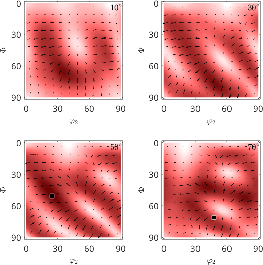
The Curl of a Vector Field
The counterpart of the flux is the curl of a vector field which describes the axis of local rotation within the crystal orientations.
From mathematics we know that the curl of a gradient field is zero
plot(G.curl,'sigma')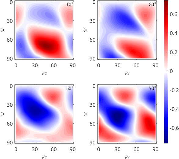
Antiderivative of a Gradient Field
The fact that the curl of a vector field is zero is actually equivalent to the fact that the vector field is the gradient of some potential field, which can be computed by the command antiderivative(g) and coincides exactly with the original ODF odf.
odf2 = G.antiderivative

plot(odf2,'sigma')
odf2 = SO3FunHarmonic (Quartz → y↑→x)
bandwidth: 48
weight: 0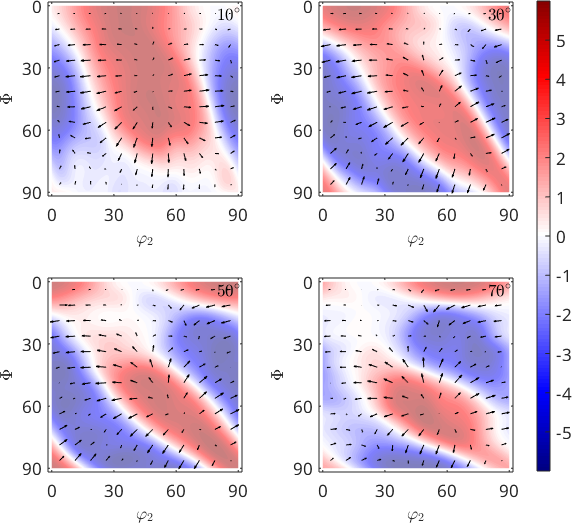
Construction of Orientational Vector Fields
Explicitly by an Anonymous Function
Analogous to SO3FunHandle we are able to define SO3VectorFields by an anonymous function.
% cubic symmetry
cs = crystalSymmetry('432')

% product of rotational axis and rotational angle
f = @(mori) axis(mori) .* angle(mori);

% define the vector field
VF = SO3VectorFieldHandle(f,cs,cs)

% evaluating the vector field gives what we expect
round(VF.eval(orientation.byAxisAngle(vector3d(1,2,3),10*degree)))
cs = crystalSymmetry
symmetry: 432
elements: 24
a, b, c : 1, 1, 1
VF = SO3VectorFieldHandle (432 → 1)
tangent space: leftVector
intern symmetries: 432 → 432
ans = SO3TangentVector (y↑→x)
intern symmetries: 432 → 432
TagentSpace: leftVector
x y z
1 2 3But plotting does not -- TODO!!!
% plot it
quiver3(VF,'axisAngle','resolution',7.5*degree,'color','black','linewidth',2)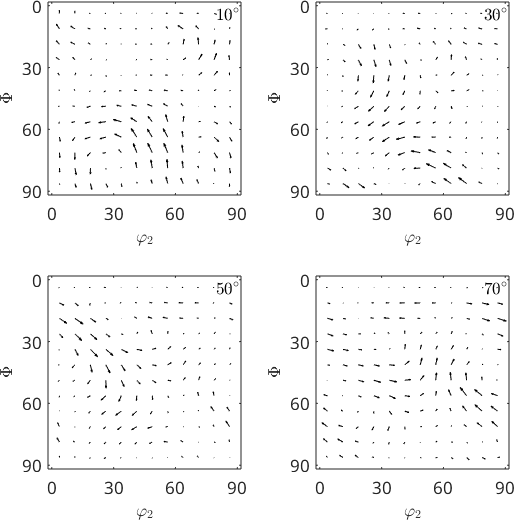
Definition via SO3VectorField
We can expand any SO3VectorField in an SO3VectorFieldHarmonic directly by the command SO3VectorFieldHarmonic
SO3VectorFieldHarmonic(VF)ans = SO3VectorFieldHarmonic (432 → 1)
bandwidth: 64
tangent space: leftVector
intern symmetries: 432 → 432Definition via function values
At first we need some example rotations
nodes = equispacedSO3Grid(specimenSymmetry('1'),'points',1e3);
nodes = nodes(:);
Next, we define function values for the rotations
y = vector3d.byPolar(sin(3*nodes.angle), nodes.phi2+pi/2);Now the actual command to get SO3VF1 of type SO3VectorFieldHarmonic
SO3VF1 = SO3VectorFieldHarmonic.approximate(nodes, y,'bandwidth',16)SO3VF1 = SO3VectorFieldHarmonic (y↑→x → y↑→x)
bandwidth: 16
tangent space: leftVectorDefinition via function handle
If we have a function handle for the function we could create a S2VectorFieldHarmonic via quadrature. At first lets define a function handle which takes rotation as an argument and returns a vector3d:
Now we can call the quadrature command to get SO3VF2 of type SO3VectorFieldHarmonic
SO3VF2 = SO3VectorFieldHarmonic.quadrature(@(v) f(v))SO3VF2 = SO3VectorFieldHarmonic (y↑→x → y↑→x)
bandwidth: 64
tangent space: leftVector
Definition via SO3FunHarmonic
If we directly call the constructor with a vector valued SO3FunHarmonic with three entries it will create a SO3VectorFieldHarmonic with SO3F(1), SO3F(2), and SO3F(3) the \(x\), \(y\), and \(z\) component.
SO3F = SO3FunHarmonic(rand(1e3, 3))
SO3VF3 = SO3VectorFieldHarmonic(SO3F)
SO3F = SO3FunHarmonic (y↑→x → y↑→x)
isReal: false
size: 3 x 1
bandwidth: 9
weights: [0.89 0.79 0.13]
SO3VF3 = SO3VectorFieldHarmonic (y↑→x → y↑→x)
isReal: false
bandwidth: 9
tangent space: leftVectorApplication: Orientation Dependent Spin Tensors as Vector Fields
According to Taylor theory the strain acting on a crystal with orientation ori is compensated by the action of different slip systems. The antisymmetric portion of deformation tensors of these active slip systems gives a spin tensors that describes the local misorientation the crystal undergoes under deformation. In MTEX the spin tensor W as a function of the orientation ori is computed as a variable of type SO3VectorField by the command calcTaylor.
% consider bcc symmetry and slip systems
cs = crystalSymmetry('432');
sS = slipSystem.bcc(cs)

% consider plane stain
q = 0;
epsilon = strainTensor(diag([1 -q -(1-q)]))

% compute the orientation depended spin tensor
[~,~,W] = calcTaylor(epsilon,sS.symmetrise)
sS = slipSystem (432)
size: 1 x 3
u v w | h k l CRSS
1 -1 1 0 1 1 1
-1 1 1 2 1 1 1
-1 1 1 3 2 1 1
epsilon = strainTensor (y↑→x)
type: Lagrange
rank: 2 (3 x 3)
1 0 0
0 0 0
0 0 -1
W = SO3VectorFieldHarmonic (1 → y↑→x)
bandwidth: 32
tangent space: rightSpinTensor
intern symmetries: 432 → y↑→x
intern tangent space: leftVectorLets visualize the spin tensor in Euler angle sections
sP = phi1Sections(cs,specimenSymmetry('222'));
sP.phi1 = (10:20:70)*degree;

% plot the Taylor factor
plot(W,sP,'resolution',7.5*degree,'layout',[2 2])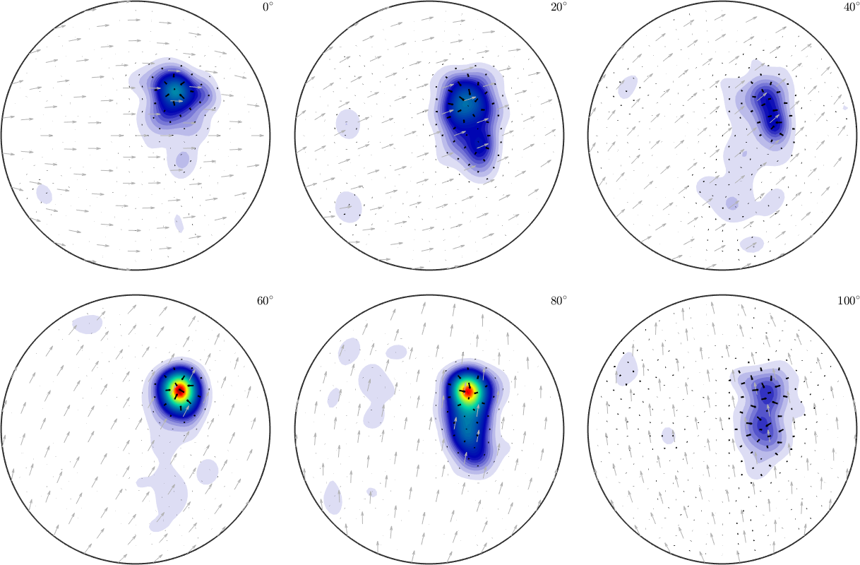
We observe how according to the orientation the Taylor model predicts a misorientation of the corresponding crystal. For a specific (set of) orientation ori we can retrieve the spin tensor by evaluating the vector field W at this position
% the spin tensor for the copper orientation
WCopper = W.eval(orientation.copper(cs))
WCopper = spinTensor (y↑→x)
rank: 2 (3 x 3)
*10^-2
0 0 32.15
0 0 32.15
-32.15 -32.15 0The Norm of a Vector Field
The norm of the spin tensor directly relates to the amount of misorientation. We may compute the amount of misorientations as a function of orientation by the command norm and determine the orientation of maximum misorientation by
% determine the orientation of maximum misorientation
[~,oriMax] = max(norm(W))

% visualize the amount of misorientation
plot(norm(W),sP,'resolution',0.5*degree,'layout',[2 2])
mtexColorMap LaboTeX

% plot the vector field on top
hold on
plot(W,sP,'resolution',7.5*degree,'color','black')
hold off

annotate(oriMax)
oriMax = orientation (432 → y↑→x)
Bunge Euler angles in degree
phi1 Phi phi2
268.696 45.4283 63.3496
As the vector field W corresponds to the rotational axis of the local misorientation we may check how much this axis corresponds with a predefined axis, e.g. [100], by computing the inner product dot(W,d) between the vector field W and the predefined axis d.
plot(dot(W,Miller(1,0,0,cs)),sP,'layout',[2 2])
mtexColorMap blue2red
mtexColorbar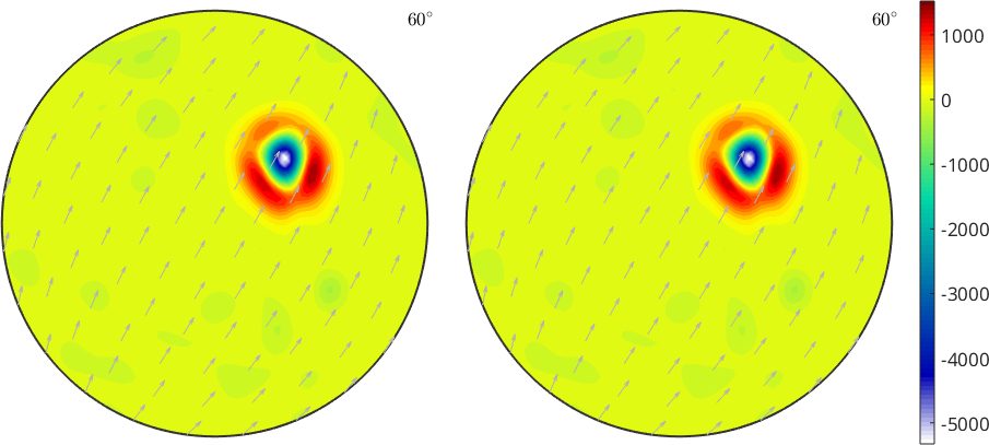
The Flux of a Vector Field
If we interpret the vector field W as a velocity field for the different crystal orientations. Then its divergence is a scalar field that indicates where orientations condense. In this interpretation a sink corresponds to negative flux / divergence and a source to positive flux / divergence.
flux = W.div

plot(flux,sP,'resolution',0.5*degree,'layout',[2 2],'faceAlpha',0.5)
mtexColorMap blue2red
mtexColorbar

hold on
plot(W,sP,'resolution',7.5*degree,'color','black')
hold off
flux = SO3FunHarmonic (432 → y↑→x)
bandwidth: 32
weight: 0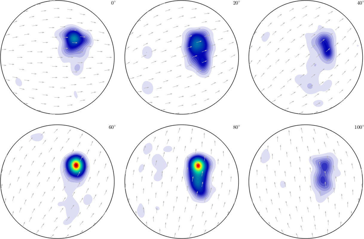
The Curl of a Vector Field
The counterpart of the flux is the curl of a vector field which describes the axis of local rotation within the crystal orientations
c = W.curl

plot(c,sP,'resolution',7.5*degree,'layout',[2 2],'color','black')
c = SO3VectorFieldHarmonic (1 → y↑→x)
bandwidth: 32
tangent space: rightSpinTensor
intern symmetries: 432 → y↑→x
intern tangent space: leftVector