Tensor Arithmetic

This page assumes the tensor ranks and physical classes introduced in Defining Tensorial Properties. It shows how MTEX applies arithmetic to one tensor or a list without loops. The central operation is a contraction: a sum over selected component indices.

The rotation examples also assume the active rotations introduced in Defining Rotations.

plottingConvention.default('y↑→x');

Basic algebra

Addition, scalar multiplication, and elementwise operations follow MATLAB array notation. These variables each contain three random rank 2 tensors, so every line below acts on all three at once.

T1 = tensor.rand(3,'rank',2);
T2 = tensor.rand(3,'rank',2);

% addition and scalar multiplication
T = T1 + 2 * T2;

% componentwise multiplication
T = T1 .* T2;

The operator .* multiplies corresponding components. It is not an outer product and does not change the rank. The random tensors are algebraic examples rather than tensors with the symmetries of a physical property.

Contractions with EinsteinSum

Hooke's law is a useful model for reading a contraction. The following rank 4 stiffness tensor contains room-temperature measurements for San Carlos olivine from Abramson et al. (1997). Importing Tensor Data explains the loading step and the reference-frame information that must accompany published components.

C = stiffnessTensor.load(fullfile(mtexDataPath,'tensor','Olivine1997PC.GPa'));

The data are in GPa. Apply a strain that stretches along x and compresses along z.

eps = strainTensor(diag([1 0 -1]))

eps = strainTensor (y↑→x)
  type: Lagrange 
  rank: 2 (3 × 3)
 
  1  0  0
  0  0  0
  0  0 -1

Hooke's law contracts the last two indices of the stiffness with the two indices of the strain,

\[\sigma_{ij} = \sum_{k,l} C_{ijkl} \epsilon_{kl}.\]

EinsteinSum takes each tensor followed by one label for each of its indices. Equal negative labels mark indices to sum over. Positive labels survive, and their values set the index order in the result. The signs are MTEX syntax; the physical indices are not negative.

sigma = EinsteinSum(C,[1 2 -1 -2],eps,[-1 -2])

sigma = tensor (y↑→x)
  rank: 2 (3 × 3)
 
  248.9      0      0
      0  -8.65      0
      0      0 -161.9

Labels 1 and 2 leave a rank 2 result. Its diagonal normal stresses are 248.9, -8.65, and -161.9 GPa; all shear components are zero.

The same notation describes elementary products. The outer product

\[ (a \otimes b)_{ij} = a_i b_j \]

has two free indices and no summation.

a = tensor([1;2;3],'rank',1);
b = tensor([0;2;1],'rank',1);

ab = EinsteinSum(a,1,b,2)

ab = tensor (y↑→x)
  rank: 2 (3 × 3)
 
 0 2 1
 0 4 2
 0 6 3

The inner product

\[ a \mathbin{\cdot} b = \sum_i a_i b_i \]

instead repeats one negative label and leaves no free index. Its result is the scalar 7.

aDotB = EinsteinSum(a,-1,b,-1)

aDotB =
     7

Stiffness is not compliance

Linear compressibility is the relative shortening along a direction v under unit hydrostatic pressure. It is a contraction of the compliance \(S=C^{-1}\),

\[ \beta(v) = \sum_{i,j,k} S_{ijkk} v_i v_j.\]

inv turns the stiffness into a compliance tensor. The data file identifies x with [100], the crystallographic a direction.

v = xvector;
S = inv(C);
beta = EinsteinSum(S,[-1 -2 -3 -3],v,-1,v,-2)

beta =
    0.0018

The result is 0.0018 GPa\(^{-1}\). It is the same contraction used by linearCompressibility.

betaDirect = C.linearCompressibility(v);

Contracting the stiffness in the same way is dimensionally wrong. The result is 460.25 GPa, not a compressibility.

wrongUnits = EinsteinSum(C,[-1 -2 -3 -3],v,-1,v,-2)

wrongUnits =
  460.2500

Named contractions

Frequently used contractions have operators. For a stiffness and a strain, both * and : apply Hooke's law. They also preserve the physical result class, so the first command displays a stressTensor rather than the generic tensor returned by EinsteinSum.

sigmaTimes = C * eps
sigmaColon = C : eps;

sigmaTimes = stressTensor (y↑→x)
  rank: 2 (3 × 3)
 
  248.9      0      0
      0  -8.65      0
      0      0 -161.9

Between two rank 2 tensors, the double dot product is their inner product. It is also the trace of either matrix product below. Each result here is a list of three scalars because T1 and T2 are lists.

inner = T1 : T2
innerFromLeftTrace = trace(T1 * T2');
innerFromRightTrace = trace(T1' * T2);

inner =
    1.2723
    2.6104
    1.7063

Rank 2 matrix operations

det returns one determinant for each rank 2 tensor in the list. The same function also supports rank 4 tensors.

d = det(T1)

d =
    0.0650
   -0.0782
    0.0251

Rotating a tensor

rotate actively rotates a physical property. The workshop example below starts with a second-rank thermal-conductivity tensor whose largest value, 10.5 W m\(^{-1}\) K\(^{-1}\), is along x. The rotation moves that preferred direction 45 degrees about z.

K = tensor(diag([10.5 6.2 6.2]),'rank',2,...
  'propertyname','thermal conductivity','unit','W m^-1 K^-1');
r = rotation.byAxisAngle(zvector,45*degree);
Krot = rotate(K,r);

newMtexFigure('layout',[1 2]);
plot(K,'complete','upper')
mtexTitle('before rotation')

nextAxis
plot(Krot,'complete','upper')
mtexTitle('after rotation')

setColorRange('equal')
mtexColorbar('title','thermal conductivity (W m^{-1} K^{-1})')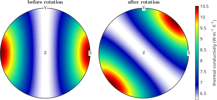

The high-conductivity region turns in the right plot, while its maximum stays 10.5. A rank 2 tensor receives one rotation matrix per index,

\[ K'_{ij} = \sum_{p,q} R_{ip} R_{jq} K_{pq}. \]

Rotating the property is not a frame change. A frame change re-expresses the same physical object in another reference frame. Use transformReferenceFrame for that operation; Reference Frame Alignment shows why the distinction matters for published crystal properties.

A third-rank example

Nye gives the following piezoelectric modulus for a crystal with one threefold axis. The two printed component tables show the same property before and after an active rotation of -45 degrees about z.

P = [ 0 0 0 .17 0   0;
      0 0 0 0   .17 0;
      0 0 0 0   0   5.17]*10^-11;

P0 = tensor(P,'rank',3,'propertyname','piezoelectric modulus')

rPiezo = rotation.byAxisAngle(zvector,-45*degree);
P45 = rotate(P0,rPiezo)

P0 = tensor (y↑→x)
  propertyname: piezoelectric modulus
  rank        : 3 (3 × 3 × 3)        
 
  tensor in compact matrix form: *10^-12
    0    0    0  1.7    0    0
    0    0    0    0  1.7    0
    0    0    0    0    0 51.7
 
P45 = tensor (y↑→x)
  propertyname: piezoelectric modulus
  rank        : 3 (3 × 3 × 3)        
 
  tensor in compact matrix form: *10^-12
     0     0     0     0   1.7     0
     0     0     0  -1.7     0     0
  51.7 -51.7     0     0     0     0

Components that were zero before the rotation are nonzero afterwards. Nothing about the crystal changed internally: the component table changed because the property now points in different specimen directions.

Next

Tensor Visualization explains the directional plot used above and the specialized plots for physical tensor classes. Anisotropic Elasticity applies these contractions to elastic moduli, energy, and wave propagation. The polycrystal step is Tensor Averages.

Further reading