Spherical axis fields

A spherical axis field assigns an axis in three-dimensional space to every direction on the sphere. An axis has no sense: the vectors \(\vec v\) and \(-\vec v\) represent the same value. Polarization directions and principal stress or strain directions are typical examples.

S2AxisField is therefore not a vector field with an arbitrary sign convention. It represents a function

\[ f\colon \mathrm{S}^2\to\mathbb{R}^3/\{\vec v\sim-\vec v\}. \]

The class S2AxisFieldHarmonic stores such a field as a spherical harmonic expansion. This page constructs that representation from sampled values and from a function handle.

plottingConvention.default('y↑→x');

Interpolate sampled axes

Begin with directions at which the field has been sampled. Turn the grid into a column so that each row of the values below belongs to one node.

nodes = equispacedS2Grid('points',600);
nodes = nodes(:);

Define one axis at every node. The 'antipodal' flag tells vector3d to identify each value with its negative.

values = vector3d(sin(5*nodes.x),1,nodes.y,'antipodal');

interpolate fits the six components of the sign-independent dyadic product described below. Limiting the bandwidth keeps only spherical harmonic degrees up to 6. Equal weights are appropriate for this uniformly spaced example grid.

sAF1 = S2AxisFieldHarmonic.interpolate(nodes,values,'bandwidth',6, ...
  'weights','equal');

plot(sAF1,'resolution',20*degree);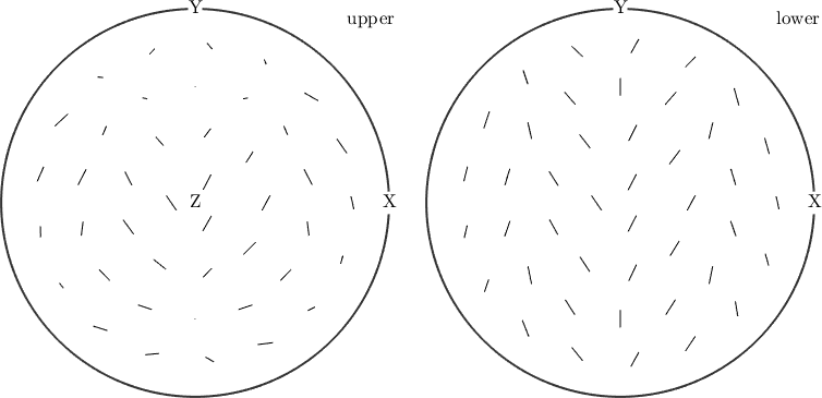

Each short black line shows the fitted axis at one plotting direction. The lines have no arrowheads because reversing any one of them would not change the field. Their gradual change across the sphere shows what the harmonic interpolation has smoothed between the sampled nodes.

Construct an axis field from a function

Use a function handle when the axis is known at every input direction. The handle must accept a vector3d array and return an equally sized antipodal vector3d array. This example makes the axes circulate around the vertical direction while a nonzero vertical component keeps the axis defined at the poles.

axisFun = @(v) vector3d(-v.y,v.x,0.35+0*v.x,'antipodal');

Passing the handle to the constructor applies spherical quadrature. The explicit equivalent is S2AxisFieldHarmonic.quadrature(axisFun,'bandwidth',6).

sAF2 = S2AxisFieldHarmonic(axisFun,'bandwidth',6);

clf;
quiver(sAF2,'resolution',20*degree);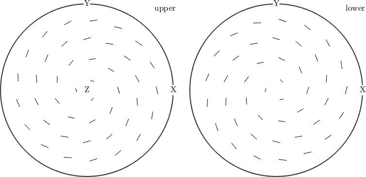

The axes now turn around the centre of the projection. Near the centre, the visible vertical component shortens their in-plane projection; this is a projection effect, not a loss of axis length. The quiver command is an alias for the default two-dimensional plot of an axis field.

Evaluate the field

Use eval to obtain the fitted axis at any direction. The result remains antipodal, so code that consumes it must not attach meaning to its displayed sign.

queryDirection = vector3d.byPolar(50*degree,35*degree);
axisAtQuery = sAF2.eval(queryDirection);

Why the sign disappears

A harmonic axis field does not expand the three components of \(\vec v\) directly. It expands the six independent entries of the symmetric dyadic product \(\vec v\vec v^{\mathrm T}\). Reversing the representative leaves this matrix unchanged because

\[(-\vec v)(-\vec v)^{\mathrm T}=\vec v\vec v^{\mathrm T}. \]

Evaluation recovers the axis as the leading eigenvector of the fitted matrix. This construction is the reason a harmonic axis field can interpolate axes without first choosing consistent signs for the input values.

close all

References

Next

Continue with Symmetric spherical functions to build a scalar spherical function whose values repeat under a chosen symmetry.