In this chapter various ways of plotting spherical functions are explained. We start by defining some example functions.
% the smiley
sF1 = S2Fun.smiley;

% some oscillatory function
f = @(v) 0.1*(v.theta+sin(8*v.x).*sin(8*v.y));
sF2 = S2FunHarmonic.quadrature(f, 'bandwidth', 150);
Smooth Plot
The default pcolor command generates a colored plot without contours. Then more general command which yields the same result is simply plot
plot(sF1)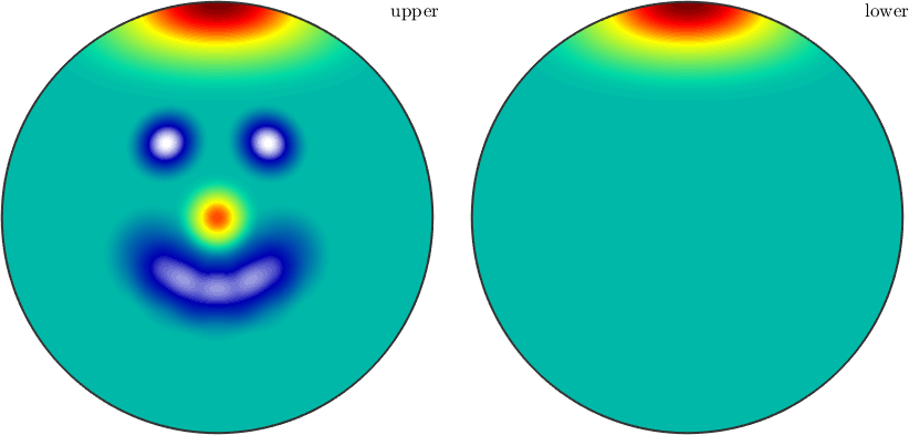
Contour Plot
Filled or non-filled contour plot can be generated by the commands contourf and contour
contour(sF1,'upper');
nextAxis(1,2)
contourf(sF1,'upper');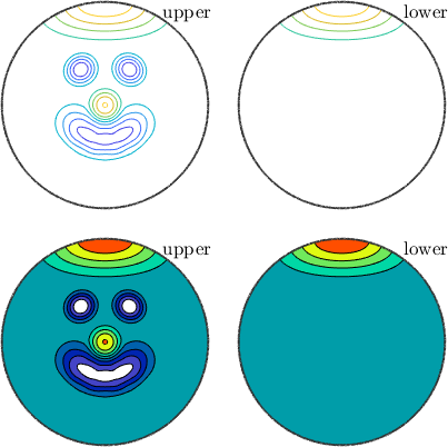
Free rotate-able 3D Plot
The command plot3d yield a three dimensional plot which can be rotated freely using the mouse.
plot3d(sF1);

how2plot = plottingConvention;
how2plot.north = xvector;
how2plot.outOfScreen = vector3d(0,1,2);
setCamera(how2plot)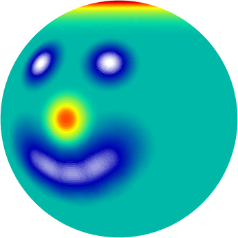
Surface Plot
3D plot where the radius of the sphere is transformed according to the function values
surf(sF1)
axis off
setCamera(how2plot)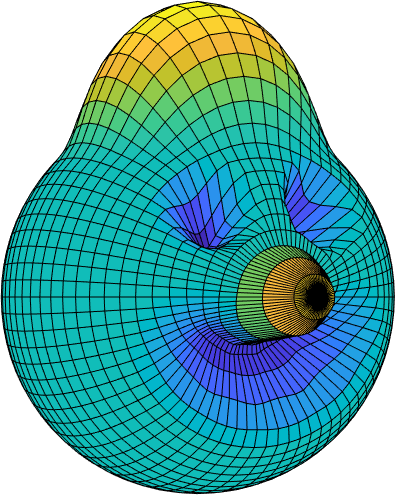
Section Plot
Plot the intersection of the surf plot with a plane defined by a normal vector N
plotSection(sF2, zvector,'color','interp','linewidth',10)
colormap spring
mtexTitle('Flowerpower!')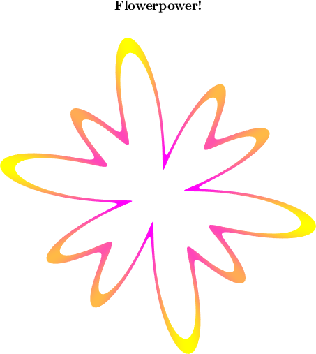
Spectral Plot
plotting the Fourier coefficients
close all
plotSpektra(sF1,'FontSize',15,'linewidth',2);
xlim([0,40])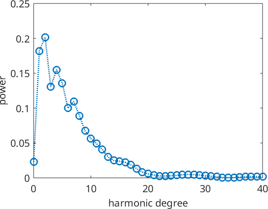
The more specific plot options are covered in the respective classes.