Reference Frame Alignment

The most important difference between MTEX and many other EBSD software is that in MTEX the Euler angle reference is always the map reference frame. This mean the \(x\) and \(z\) axes of the map are exactly the rotation axes of the Euler angles.

In case the map coordinates and the Euler angles in your data are with respect to different reference frames it is highly recommended to correct for this while importing the data into MTEX. This section explains in detail how to do this.

On Screen Orientation of the EBSD Map

Many people are concerned when the images produced by MTEX are not aligned exactly as they are in their commercial software. It is indeed very important to understand exactly the alignment of your data. However, the important point is not whether a map is upside down on your screen or not. The important point is how your map aligns with the specimen, as we want to use the map to describe properties of the specimen.

There are basically two components in an EBSD data set that refer to the specimen reference frame: the spatial coordinates \(x\), \(y\) and the Euler angles \(\phi_1\), \(\Phi\), \(\phi_2\). To explain the difference have a look at the EDAX export dialog

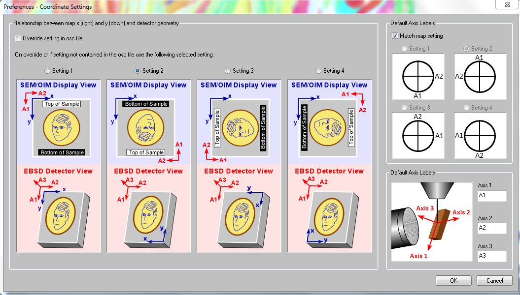
Here we have the axes \(x\) and \(y\) which describe how the map coordinates needs to be interpreted and the axes \(A_1\), \(A_2\), \(A_3\) which describe how the Euler angles, and in consequence, the pole figures needs to be interpreted. We see that in none of these settings the map reference system coincides with the Euler angle reference frame.

This situation is not specific to EDAX but occurs as well with EBSD data from Oxford or Bruker, all of them using different reference system alignments. For that reason MTEX strongly recommends to transform the data such that both map coordinates and Euler angles refer to the same coordinate system.

Doing this we have two choices:

In the case of EDAX data imported from an *.ang file we still need to specify the export option used by the EDAX software. This is done by the options 'setting 1', 'setting 2', 'setting 3' or 'setting 4'.

Since setting 2 is default for most EDAX exports a typical command for importing data from an ang file would look like this

ebsd = EBSD.load([mtexEBSDPath filesep 'olivineopticalmap.ang'],...
  'convertEuler2SpatialReferenceFrame','setting 2')

plot(ebsd('olivine'),ebsd('olivine').orientations,'coordinates','on')

ebsd = EBSD
 
 Phase  Orientations       Mineral         Color  Symmetry  Crystal reference frame
     1   44953 (90%)       olivine  LightSkyBlue       222                         
     2   1370 (2.8%)      Dolomite  DarkSeaGreen         3       X||a, Y||b*, Z||c*
     3   2311 (4.6%)     Enstatite     Goldenrod       222                         
     4   1095 (2.2%)  Chalcopyrite    LightCoral       422                         
 
 Properties: ci, fit, iq, sem_signal, unknown1, unknown2, unknown3, unknown4
 Scan unit : um
 X x Y x Z : [0 888] x [0 888] x [0 0]
 Normal vector: (0,0,1)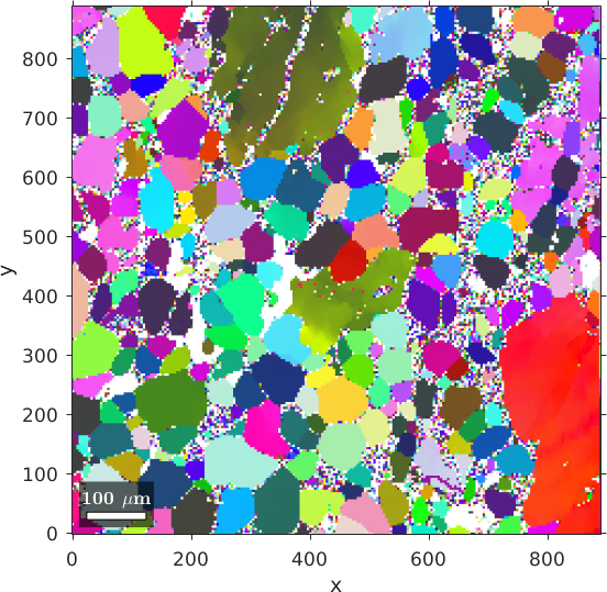

The plot does not yet fit the alignment of the map in the EDAX software as it plots the x-axis be default to east and the z-axis into the plane. This is only a plotting convention and can be set in MTEX by

ebsd.how2plot.east = xvector;
ebsd.how2plot.outOfScreen = -zvector;

plot(ebsd('olivine'),ebsd('olivine').orientations,'coordinates','on')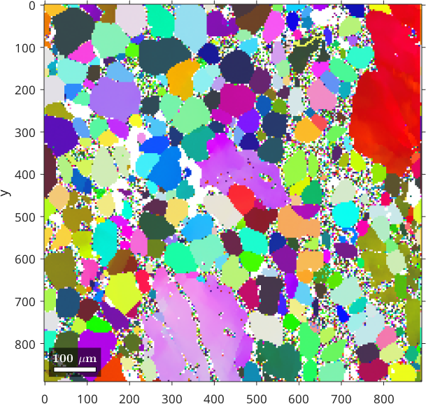

Note that these options only alter the orientation of the EBSD map and the pole figures on the screen but does not change any data.

Verify the reference system

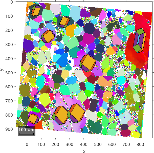
One way of verifying the reference systems is to visualize crystal shapes on top of the orientation map. To do this we proceed as follows

% reconstruct grains
grains = calcGrains(ebsd('indexed'));

% chose the correct crystal shape (cubic, hex are generic forms)
cS = crystalShape.olivine;

% select only large grains
largeGrains = grains(grains.grainSize>500)

% and plot the crystal shapes
hold on
plot(largeGrains,cS,'colored')
hold off
legend off

largeGrains = grain2d
 
 Phase  Grains  Pixels  Mineral  Symmetry  Crystal reference frame
     1       8    9556  olivine       222                         
 
 boundary segments: 2041 (7935 µm)
 inner boundary segments: 2 (8 µm)
 triple points: 582
 
   Id   Phase   Pixels       meanRotation      GOS
 1215       1      508     (11°,117°,42°)   0.0045
 1684       1      510    (201°,111°,37°)   0.0058
 2911       1      708     (48°,66°,193°)    0.046
 3954       1     3199     (133°,6°,322°)     0.05
 5018       1     1191     (25°,58°,191°)    0.056
 9750       1      502   (108°,120°,182°)   0.0028
 9761       1     1463      (26°,53°,23°)    0.088
 9768       1     1475      (26°,53°,19°)    0.091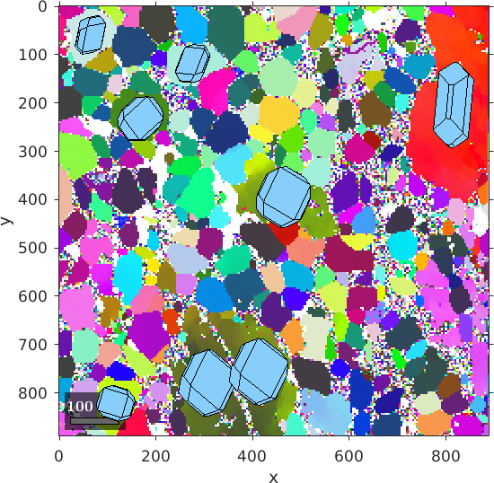

It may also be helpful to inspect pole figures

h = Miller({1,0,0},{0,1,0},{0,0,1},ebsd('O').CS);
plotPDF(ebsd('O').orientations,h,'contourf')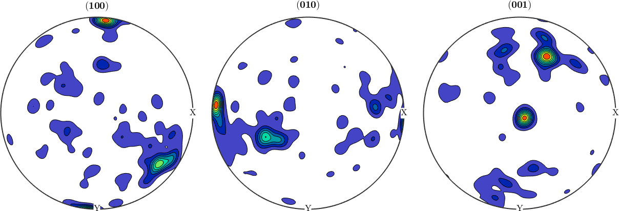

As pole figures display data relative to the specimen reference frame MTEX automatically aligns them on the screen exactly as the spatial map above, i.e., according to our last definition with x pointing towards east and y to the south.

Change the map reference system

In order to manually change the map reference frame one may apply a rotation to the map coordinates only. E.g. to flip the map left to right while preserving the Euler angles one can do

rot = rotation.byAxisAngle(yvector,180*degree);
ebsd_rot = rotate(ebsd,rot,'keepEuler');

% reconstruct grains
grains = calcGrains(ebsd_rot('indexed'));

% select only large grains
largeGrains = grains(grains.grainSize>500);

plot(ebsd_rot('olivine'),ebsd_rot('olivine').orientations,'coordinates','on')

% and plot the crystal shapes
hold on
plot(largeGrains,cS,'colored')
legend off
hold off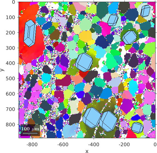

Change the Euler angle reference system

Analogously we may change the Euler angle reference frame while keeping the map coordinates

ebsd_rot = rotate(ebsd,rot,'keepXY');

% reconstruct grains
grains = calcGrains(ebsd_rot('indexed'));

% select only large grains
largeGrains = grains(grains.grainSize>500);


plot(ebsd_rot('olivine'),ebsd_rot('olivine').orientations,'coordinates','on')

% and plot the crystal shapes
hold on
plot(largeGrains,cS,'colored')
legend off
hold off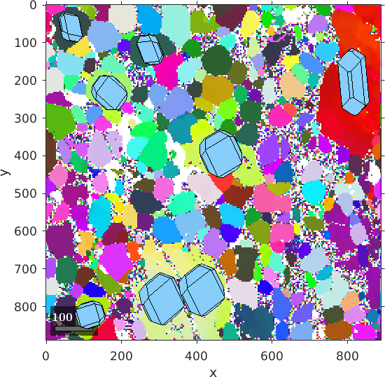

Changing both reference system simultaneously

Sometimes it is necessary to relate the EBSD data to a different external reference frame, or to change the external reference frame from one to the other, e.g. if one wants to concatenate several ebsd data sets where the mounting was not done in perfect coincidence. In these cases the data has to be rotated or shifted by the commands rotate and shift. The following commands rotate both reference frames of the entire data set by 5 degree about the z-axis.

% define a rotation
rot = rotation.byAxisAngle(zvector,5*degree);

% rotate the EBSD data
ebsd_rot = rotate(ebsd,rot);

% reconstruct grains
grains = calcGrains(ebsd_rot('indexed'));

% select only large grains
largeGrains = grains(grains.grainSize>500);


plot(ebsd_rot('olivine'),ebsd_rot('olivine').orientations,'coordinates','on')

% and plot the crystal shapes
hold on
plot(largeGrains,cS,'colored')
legend off
hold off