Random Sampling

An orientation distribution function describes a continuous population of orientations. This page solves the reverse problem to density estimation: it turns an ODF into a finite list of orientations that represents that population. The ODF may have been built as a model or reconstructed from pole-figure measurements.

There are two different reasons to do this. A random sample represents sampling variability, for example in a bootstrap or a synthetic measurement. An optimized sample represents the ODF with as few points as possible, for example as input to a crystal-plasticity calculation. These point sets may look similar, but they are not interchangeable. Sampling from a model also gives a known answer for testing a density estimation method. Crystal-plasticity codes such as VPSC also consume orientation lists in this form.

The examples use a trigonal ODF made from a randomly chosen fibre on a uniform background.

cs = crystalSymmetry('32');
fibre_odf = 0.5*uniformODF(cs) + ...
  0.5*fibreODF(fibre.rand(cs),'halfwidth',20*degree);

Draw a Random Sample

discreteSample draws orientations with probability proportional to the ODF. Each orientation in the returned list has the same implicit weight, \(1/500\) in this example.

ori = fibre_odf.discreteSample(500);

% plot the ODF in Bunge sections
plot(fibre_odf,'sections',6,'silent')
mtexColorbar('title','mrd')

% plot the sampled orientations on top
hold on
plot(ori,'MarkerFaceColor','none','all','MarkerEdgeColor','k','MarkerSize',4)
hold off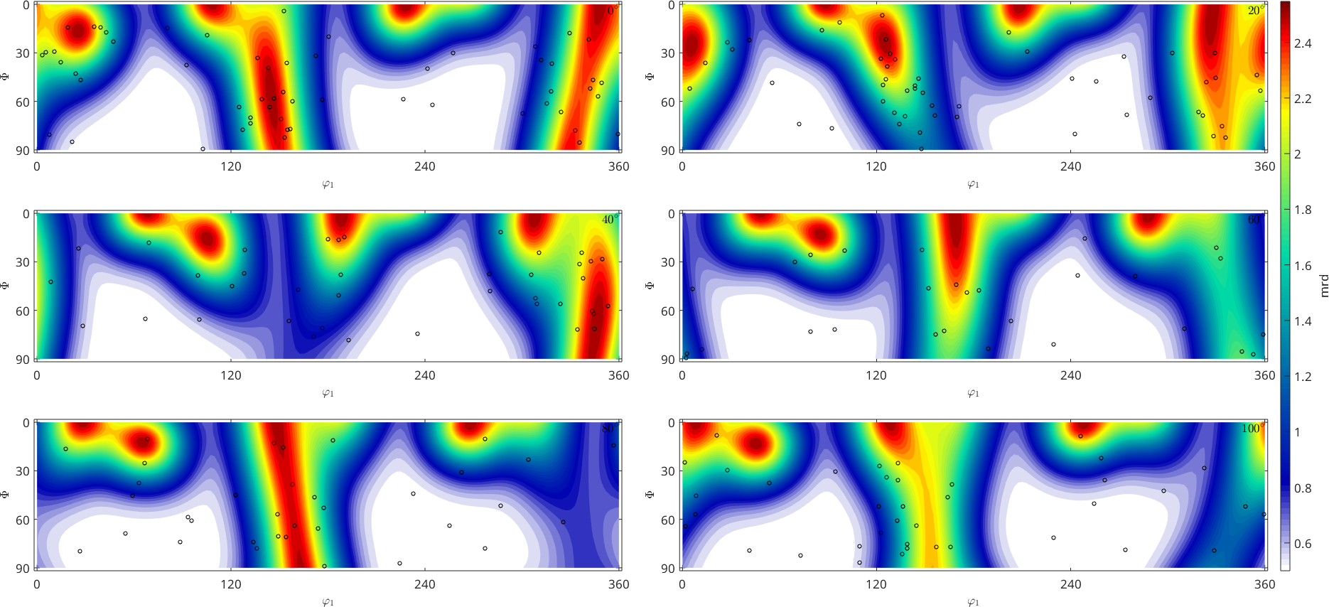

The black circles gather around the high-density parts of the coloured ODF. Their apparent crowding is not a statistical test, however. Section coordinates and projections distort area, while an ODF lives in a three-dimensional orientation space.

Sigma sections organize this trigonal example more directly and make the fibre easier to follow. They provide a better visual comparison, but they do not remove the need for a quantitative error measure.

% plot the ODF in sigma sections
plot(fibre_odf,'sections',6,'silent','sigma','contour','linewidth',2)

% plot the sampled orientations in the same sections
hold on
plot(ori,'MarkerFaceColor','none','all','MarkerEdgeColor','k','MarkerSize',4)
hold off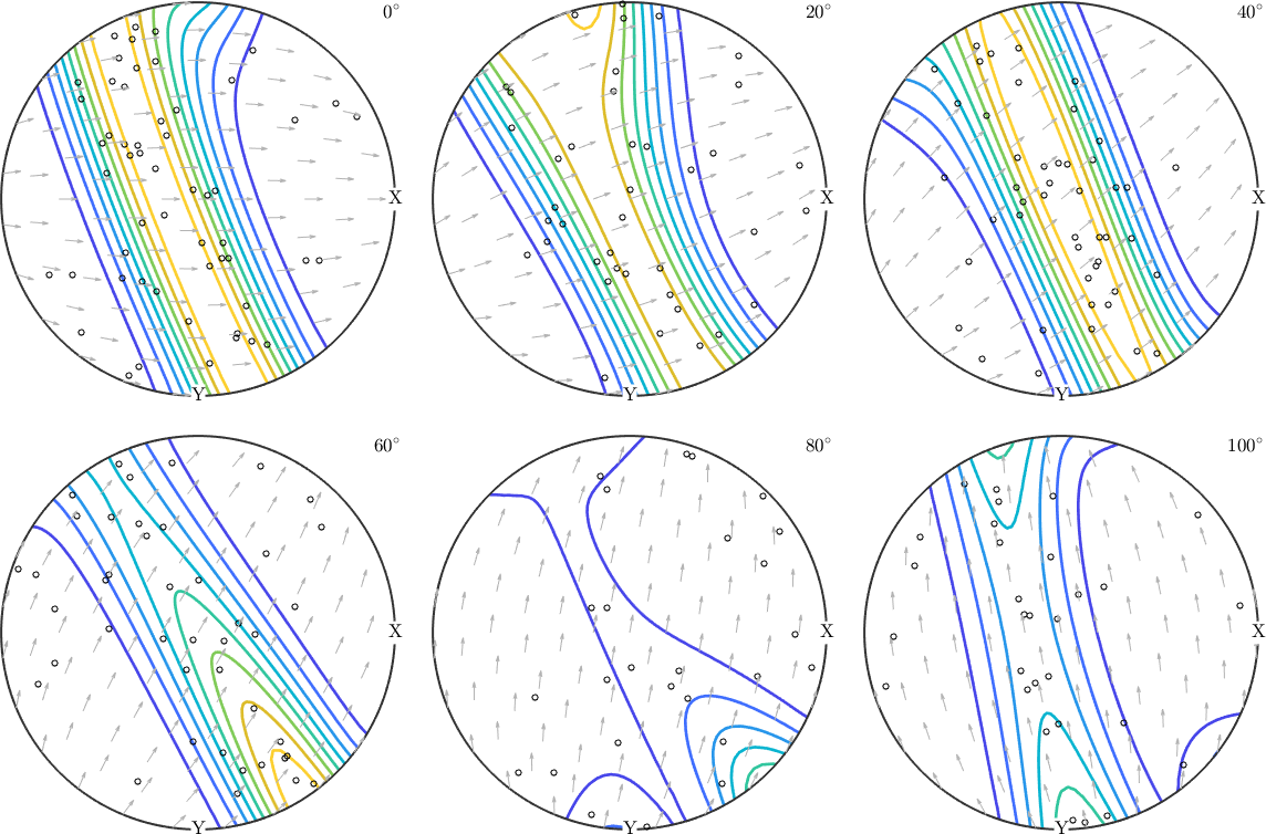

In the sigma sections, the black points trace the elongated high-density feature rather than filling orientation space uniformly. Random clusters and gaps remain because this is only one realization of 500 points.

Reconstruct the ODF from the Random Sample

A reconstruction converts the point set back to an ODF. Comparing it with the known model measures how well the sample represents the original. Here calcError is asked explicitly for the \(L^1\) error. The sample-size experiment below uses relative \(L^2\) error because that norm is cheap for harmonic ODFs. Compare errors within each experiment, not across the two different norms.

The reconstruction also introduces a kernel halfwidth. A small halfwidth retains sample-scale variation; a large one smooths that variation but also broadens real texture features.

% estimate an ODF with a narrow kernel
odf_rec = calcDensity(ori,'halfwidth',10*degree);

plot(odf_rec,'sigma','silent')
mtexColorbar('title','mrd')

errRandom10 = calcError(odf_rec,fibre_odf,'L1');
fprintf('L1 error, random sample, 10 degree: %.3f\n',errRandom10)

L1 error, random sample, 10 degree: 0.153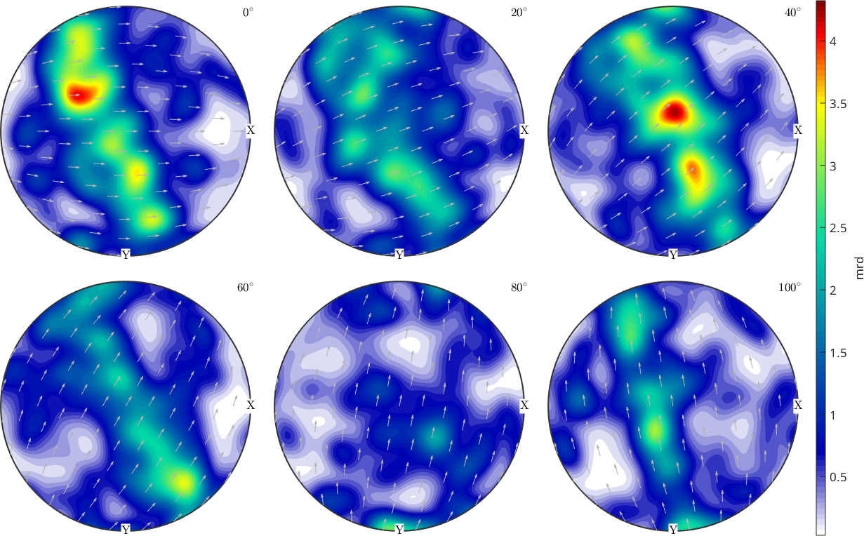

At \(10^\circ\), individual clusters and gaps appear as narrow peaks and troughs. The reconstruction shows the finite sample at least as strongly as it shows the underlying fibre.

% reconstruct the same orientations with a wider kernel
odf_rec = calcDensity(ori,'halfwidth',20*degree);

plot(odf_rec,'sigma','silent')
mtexColorbar('title','mrd')

errRandom20 = calcError(odf_rec,fibre_odf,'L1');
fprintf('L1 error, random sample, 20 degree: %.3f\n',errRandom20)

L1 error, random sample, 20 degree: 0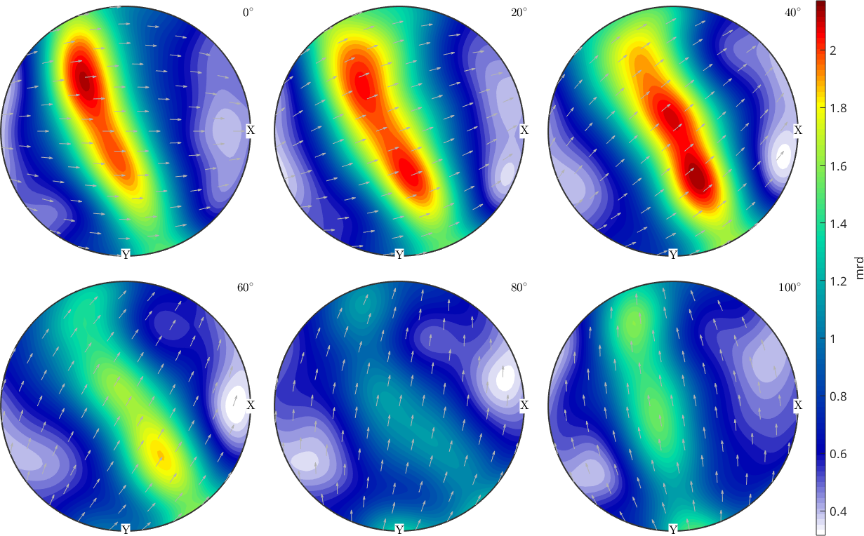.082

At \(20^\circ\), the estimate is smoother and closer to the original for this realization. The price is sharpness: the wider kernel smooths the real fibre as well as the sampling noise. Compare both the error and the texture index rather than choosing the most visually pleasing plot.

fprintf('texture index, original ODF: %.3f\n',norm(fibre_odf)^2)
fprintf('texture index, random reconstruction: %.3f\n',norm(odf_rec)^2)

texture index, original ODF: 1.351
texture index, random reconstruction: 1.220

Place an Optimized Sample

Random points are appropriate when the realization itself is part of the experiment, such as a bootstrap study of measurement accuracy. When the aim is instead a compact numerical representation, use optimalSample. It moves the orientations to reduce their discrepancy from the ODF rather than drawing independent observations.

ori = fibre_odf.optimalSample(500);

Reconstruct the optimized points with the same \(10^\circ\) halfwidth that left sample-scale peaks in the random reconstruction.

odf_rec = calcDensity(ori,'halfwidth',10*degree);

plot(odf_rec,'sigma','silent')
mtexColorbar('title','mrd')

errOptimal10 = calcError(odf_rec,fibre_odf,'L1');
fprintf('L1 error, optimized sample, 10 degree: %.3f\n',errOptimal10)

L1 error, optimized sample, 10 degree: 0.03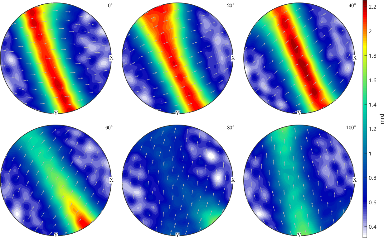9

The optimized points cover the model more evenly and support a sharper reconstruction at the same sample size. This usually reduces the error, but it does not turn the points into random observations. Use random samples to model variability and optimized samples as compact numerical input.

fprintf('texture index, original ODF: %.3f\n',norm(fibre_odf)^2)
fprintf('texture index, optimized reconstruction: %.3f\n',norm(odf_rec)^2)

texture index, original ODF: 1.351
texture index, optimized reconstruction: 1.271

Optimizing the Weights Too

The sample above gives every orientation the same weight. Requesting a second output also optimizes the weights,

[ori,c] = odf.optimalSample(500)

The nonnegative weights sum to one and are volume fractions. Pass them to the reconstruction as calcDensity(ori,'weights',c). The ODF is then represented by a weighted sum of point masses. Optimizing one weight per orientation adds degrees of freedom, so fewer orientations can represent the same ODF to a given accuracy.

Whether weighted points help depends on the reconstruction halfwidth and on the harmonic bandwidth used by optimalSample. The bandwidth says which harmonic degrees the optimization controls. Choose it for the intended use of the points; the optimalSample reference gives the details.

How Sample Size Changes the Best Halfwidth

The comparison above fixed both the sample size and the reconstruction halfwidth. A fair comparison over several sizes must tune the halfwidth separately for every sample. The following controlled experiment gives each point set the kernel that minimizes its relative \(L^2\) error, then compares the resulting errors.

The search bracket reaches to 80 degrees, well above the halfwidth any of these sample sizes calls for. A bracket that the smallest samples can reach would clip their optimum and bias the fitted laws.

These fitted laws describe this model ODF over the tested sizes. They are not universal prescriptions for another texture.

% a harmonic representation makes repeated L2 errors cheap to evaluate
odfH = SO3FunHarmonic(fibre_odf);

M = 2.^(5:9);  % 32, 64, ... 512 orientations
nRep = 5;      % independent random samples at each size

hwRand = zeros(length(M),nRep); eRand = hwRand;
hwOpt = zeros(length(M),1); eOpt = hwOpt;

for i = 1:length(M)

  % repeat the random sample because each realization differs
  for j = 1:nRep
    oriR = discreteSample(odfH,M(i));
    err = @(hw) norm(odfH - ...
      calcDensity(oriR,'halfwidth',hw*degree))/norm(odfH);
    [hwRand(i,j),eRand(i,j)] = ...
      fminbnd(err,2.5,80,optimset('TolX',0.1));
  end

  % the optimized sample is deterministic, so one run is enough
  oriO = optimalSample(odfH,M(i));
  err = @(hw) norm(odfH - ...
    calcDensity(oriO,'halfwidth',hw*degree))/norm(odfH);
  [hwOpt(i),eOpt(i)] = fminbnd(err,2.5,80,optimset('TolX',0.1));

end

Fit the Halfwidth Laws

Both optimal halfwidths are fitted by a power law,

\[\delta = a M^b,\]

using a linear fit on logarithmic coordinates.

powerLaw = @(y) polyfit(log(M(:)),log(y(:)),1);

pHwRand = powerLaw(mean(hwRand,2));
pHwOpt = powerLaw(hwOpt);

fprintf('halfwidth for discreteSample: %.1f degree * M^%.3f\n',...
  exp(pHwRand(2)),pHwRand(1))
fprintf('halfwidth for optimalSample: %.1f degree * M^%.3f\n',...
  exp(pHwOpt(2)),pHwOpt(1))

halfwidth for discreteSample: 92.9 degree * M^-0.279
halfwidth for optimalSample: 51.7 degree * M^-0.271

Plot the measured halfwidths with their fitted laws. The circles are the means of five random realizations, and the squares are the deterministic optimized samples.

Mf = logspace(log10(M(1)),log10(M(end)),100);
evalLaw = @(p,x) exp(polyval(p,log(x)));
cRand = ind2color(1); cOpt = ind2color(2);

% avoid adding this ordinary MATLAB plot to a leftover MTEX figure tile
figure

loglog(Mf,evalLaw(pHwRand,Mf),'LineWidth',1.5,'Color',cRand)
hold on
loglog(Mf,evalLaw(pHwOpt,Mf),'LineWidth',1.5,'Color',cOpt)
loglog(M,mean(hwRand,2),'o','MarkerSize',8,'Color',cRand,...
  'MarkerFaceColor',cRand)
loglog(M,hwOpt,'s','MarkerSize',8,'Color',cOpt,...
  'MarkerFaceColor',cOpt)
hold off
xlabel('number of orientations M')
ylabel('optimal halfwidth in degree')
legend('discreteSample','optimalSample','Location','southwest')
grid on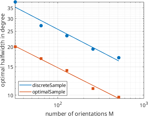

Both curves fall as the sample grows, and the optimized points lie below the random ones throughout. The random halfwidth falls the faster of the two, so the gap narrows: an optimized sample supports a much sharper kernel at the smallest size and a moderately sharper one at the largest.

fprintf('ratio of optimized to random halfwidth: %.2f at M = %d and %.2f at M = %d\n',...
  hwOpt(1)/mean(hwRand(1,:)),M(1),...
  hwOpt(end)/mean(hwRand(end,:)),M(end))

ratio of optimized to random halfwidth: 0.53 at M = 32 and 0.57 at M = 512

The Asymptotic Halfwidth Rule

For comparison, the 'magicRule' in calcKernel sets the parameter of the de la Vallee Poussin kernel to \(\kappa \sim M^{2/7}\). Since its halfwidth behaves like \(\delta \sim \kappa^{-1/2}\), the rule corresponds to \(\delta \sim M^{-1/7} \approx M^{-0.14}\).

This is the classical asymptotic kernel-density rate on a three-dimensional space. The fitted exponents above are steeper without contradicting that result: they cover less than two decades of \(M\) and a model ODF that is half uniform. The comparison between the samplers is the useful result because both were measured in the same way.

The halfwidth rules in calcKernel are derived for random samples. They will therefore oversmooth an optimized sample.

Approximation Error versus Sample Size

Once every sample has its own optimal halfwidth, compare the minimum relative \(L^2\) errors and fit a power law to each sampler.

pERand = powerLaw(mean(eRand,2));
pEOpt = powerLaw(eOpt);

figure

loglog(Mf,evalLaw(pERand,Mf),'LineWidth',1.5,'Color',cRand)
hold on
loglog(Mf,evalLaw(pEOpt,Mf),'LineWidth',1.5,'Color',cOpt)
loglog(M,mean(eRand,2),'o','MarkerSize',8,'Color',cRand,...
  'MarkerFaceColor',cRand)
loglog(M,eOpt,'s','MarkerSize',8,'Color',cOpt,...
  'MarkerFaceColor',cOpt)
hold off
xlabel('number of orientations M')
ylabel('relative L^2 error of the reconstruction')
legend('discreteSample','optimalSample','Location','southwest')
grid on

fprintf('error for discreteSample: %.2f * M^%.3f\n',...
  exp(pERand(2)),pERand(1))
fprintf('error for optimalSample: %.2f * M^%.3f\n',...
  exp(pEOpt(2)),pEOpt(1))

error for discreteSample: 0.83 * M^-0.190
error for optimalSample: 0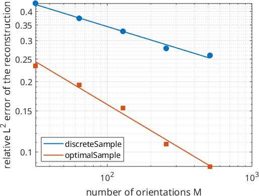.88 * M^-0.370

The optimized sample has the steeper fitted slope here too, and therefore converges faster over this tested range.

Equating the fitted laws estimates how many random orientations are needed to match an optimized set of size \(M\).

nEquiv = @(m) exp((polyval(pEOpt,log(m)) - pERand(2))/pERand(1));

for m = M
  fprintf('%d optimized orientations correspond to %.0f random ones\n',...
    m,nEquiv(m))
end

32 optimized orientations correspond to 618 random ones
64 optimized orientations correspond to 2379 random ones
128 optimized orientations correspond to 9163 random ones
256 optimized orientations correspond to 35289 random ones
512 optimized orientations correspond to 135899 random ones

Limits of the Comparison

These numbers belong to the model ODF on this page. Neither prefactors nor exponents carry over unchanged to another ODF. The prefactors scale with the halfwidth of the true ODF, and the fitted exponents become flatter for a sharper texture.

The robust qualitative result is the structure of the comparison: the best halfwidths have similar exponents, while the optimized sample works with a kernel about one third sharper in this experiment. Its advantage is also limited by the harmonic bandwidth used during optimization. Once a reconstruction depends on degrees beyond that bandwidth, the optimization no longer controls its error and the curves approach each other again.

Exporting the Orientations

A sampled orientation list can be exported as Euler angles with export. Crystal-plasticity programs often require a particular convention and a weight in every row. Use export_VPSC for the VPSC format.

The broader choice between exact ODF storage, tabulated function values, and weighted orientation lists is covered in ODF Export.

Further Reading

Next

ODF Export writes an ODF or its finite representation to a file. Density Estimation develops the inverse step from orientations to a density, while Optimal Kernel Selection compares data-driven halfwidth rules for random measurements.