This code demonstrates how clustering algorithms can be used to separate sets of vectors, crystal directions or orientations into groups by proximity.
define a cubic crystal symmetry
cs  = crystalSymmetry('432');

% define an ODF with two radial peaks
ori = orientation.byEuler([10 40]*degree,[30 50]*degree,[50 70]*degree,cs)
odf = unimodalODF(ori,'halfwidth',5*degree);

% view the odf
plotPDF(odf,Miller(1,0,0,odf.CS),'contour','linewidth',2);

% generate 10k orientations from this randomly defined ODF function
ori = odf.discreteSample(1000);

% convert the orientations to vector3d
r = ori.symmetrise * Miller(1,0,0,odf.CS);
ori = orientation (432 → y↑→x)
size: 1 x 2
Bunge Euler angles in degree
phi1 Phi phi2
10 30 50
40 50 70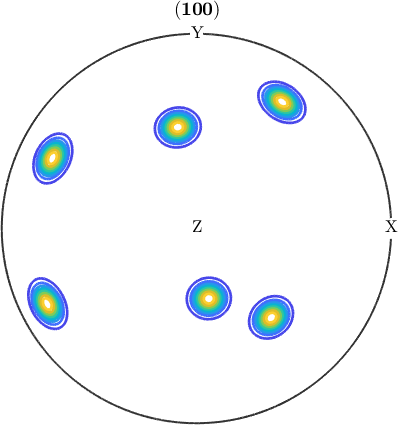
assign each vector to one of twelve clusters and calculate the center of each cluster
[cId,center] = calcCluster(r,'numCluster',12);

% plot the clusters, sorted by color
plot(r,ind2color(cId),'MarkerSize',4,'MarkerAlpha',0.02)

% annotate all the cluster centers, on all figures.
annotate(center,'add2all');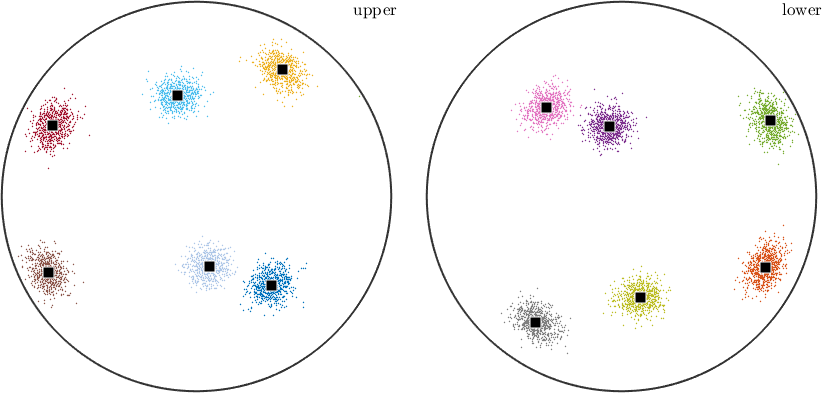
Note that the upper and lower hemisphere plots are versions of each other, reflected horizontally plus vertically. This means that the underlying data has antipodal symmetry, contributing equally to both hemispheres. Let's include that in the cluster sorting.
repeat the calculation after changing all the vector3d to be antipodal
r.antipodal = true;

% repeat the calculation assigning the vectors to clusters.  Due to the
% increased symmetry there are only six clusters now.
[cId,center] = calcCluster(r,'numCluster',6);

% plot the vectors.  Note that we no longer get an upper and lower
% hemisphere plot; the antipodal symmetry tells MTEX they are equivalent
% and so one sufficient to represent the data.

plot(r,ind2color(cId),'MarkerSize',4,'MarkerAlpha',0.01)

% annotate the cluster centers.
annotate(center,'add2all')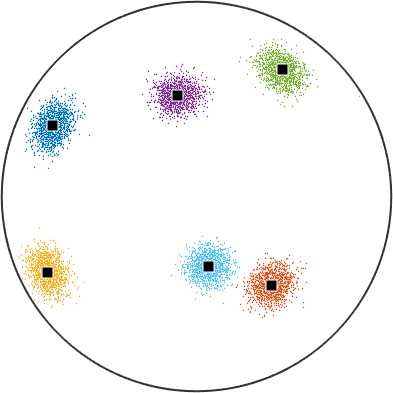
pick a vector3d, and use that to convert the 10k random orientations previously generated into crystal directions.
h = ori \ vector3d(1,1,0);

% assign the crystal directions to two clusters
[cId,center] = calcCluster(h,'numCluster',2);

% plot the crystal symmetry data on appropriate fundamental sector
plot(h.project2FundamentalRegion,ind2color(cId),'fundamentalSector',...
  'MarkerSize',4,'MarkerAlpha',0.5)

% annotate the cluster centers
annotate(center,'add2all')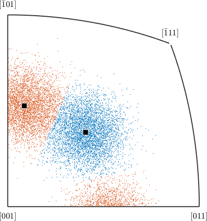
just as we calculated clusters for vectors and crystal directions, we're now going to do so for orientations
[cId,center] = calcCluster(ori,'numCluster',2,'method','hierarchical');

% create a pole figure of the orientations colored by the cluster they
% belong to.
plotPDF(ori,ind2color(cId),Miller(1,0,0,cs),'all','MarkerSize',5,...
  'MarkerAlpha',0.01)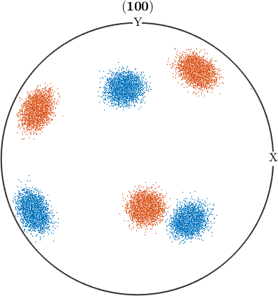
If you have the statistics toolbox, you can make some calculations about the spread of points assigned to each cluster.
r = discreteSample(r,2000)

% compute the full distance matrix between all combinations of vectors
d = angle_outer(r,r);
% convert all small values to zero to simplify later calculations
d(d<0.01) = 0;
%d = d(triu(true(size(d)),1));

% use the statistic toolbox
try
  d = squareform(d);
  z = linkage(d,'ward');

  %cId = cluster(z,'cutoff',30*degree);
  cId = cluster(z,'maxclust',6);

  plotCluster(r,cId,'MarkerSize',4,'MarkerAlpha',0.1)
catch
  warning('Statistics Toolbox not installed!')
end
r = vector3d (y↑→x)
size: 2000 x 1
antipodal: true
Warning: ward's linkage specified with non-Euclidean
dissimilarity matrix.function plotCluster(r,cId,varargin)
scatter(r(cId==1),'MarkerFaceColor',ind2color(1),varargin{:})
hold on
for i = 2:max(cId)
scatter(r(cId==i),'add2all','MarkerFaceColor',ind2color(i),varargin{:})
end
hold off
end