Operations on Crystal Directions

Operations on Crystal Directions edit page

In this section we discuss basic operations with lattice directions and lattice planes. Lets start by importing and plotting a simulated Quartz Kikuchi pattern

data = load([mtexDataPath filesep 'quartzPattern.mat']);
pattern = data.pattern;

[~,ax1] = plot(pattern,'resolution',0.25*degree,'complete','upper',"uvw");
mtexColorMap black2white
nextAxis
[~,ax2] = plot(pattern.radon,'resolution',0.25*degree,'complete','upper','hkl');
mtexColorMap black2white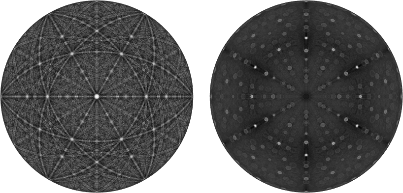

Next we consider the most reflective lattice planes in Quartz which are the positive and negative rhomboedron planes as well as the hexagonal prism planes

% extract the crystal symmetry
cs = pattern.CS;

m = Miller(-1,0,1,0,cs,'hkil'); % hexagonal prism
r = Miller(0,-1,1,1,cs,'hkil'); % positive rhomboedron
z = Miller(0,1,-1,1,cs,'hkil'); % negative rhomboedron

and visualize them as planes in the Kikuchi pattern and as points in the dual pattern

hold on
circle(m,'parent',ax1,'color','lightBlue')
circle(r,'parent',ax1,'color','red')
circle(z,'parent',ax1,'color','yellow')

opt = {'marker','s','MarkerFaceColor','none','parent',ax2,...
  'labeled','backgroundColor','w','linewidth',2};
plot(m,opt{:},'markerEdgeColor','lightBlue')
plot(r,opt{:},'markerEdgeColor','red')
plot(z,opt{:},'markerEdgeColor','yellow')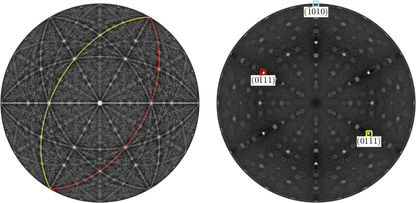

Symmetrically Equivalent Planes and Directions

Since crystal lattices are symmetric lattice directions can be grouped into classes of symmetrically equivalent directions. Those groups can be derived by permuting the Miller indices (uvw). The class of all directions symmetrically equivalent to (uvw) is commonly denoted by \(uvw\), while the class of all lattice planes symmetrically equivalent to the plane (hkl) is denoted by {hkl}. Given a lattice direction or a lattice plane all symmetrically equivalent directions and planes are computed by the command symmetrise

symmetrise(r)

ans = Miller (alpha-quartz low)
 size: 6 x 1
   h  k  i  l
   0 -1  1  1
   0  1 -1 -1
   1  0 -1  1
   1 -1  0 -1
  -1  1  0  1
  -1  0  1 -1

Lets add all symmetrically equivalent planes and directions on top of the Kikuchi pattern. Note that you may also use the options 'symmetrise' together with the plot command.

hold on
circle(m.symmetrise,'parent',ax1,'color','lightBlue')
circle(r.symmetrise,'parent',ax1,'color','red')
circle(z.symmetrise,'parent',ax1,'color','yellow')

plot(m,opt{:},'markerEdgeColor','lightBlue','symmetrised')
plot(r,opt{:},'markerEdgeColor','red','symmetrised')
plot(z,opt{:},'markerEdgeColor','yellow','symmetrised')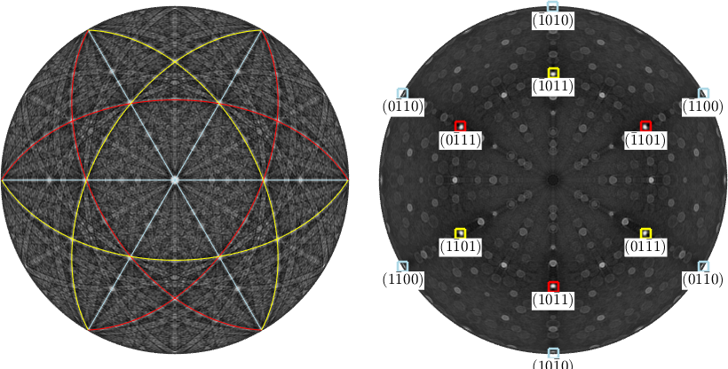

As always the keyword 'antipodal' adds antipodal symmetry

symmetrise(r,'antipodal')

ans = Miller (alpha-quartz low)
 size: 12 x 1
   h  k  i  l
   0 -1  1  1
   0  1 -1 -1
   0  1 -1 -1
   0 -1  1  1
   1  0 -1  1
  -1  0  1 -1
   1 -1  0 -1
  -1  1  0  1
  -1  1  0  1
   1 -1  0 -1
  -1  0  1 -1
   1  0 -1  1

The command eq or == can be used to check whether two crystal directions are symmetrically equivalent. Compare

Miller(1,1,-2,0,cs) == Miller(-1,-1,2,0,cs)

ans =
  logical
   0

and

eq(Miller(1,1,-2,0,cs),Miller(-1,-1,2,0,cs),'antipodal')

ans =
  logical
   1

Zone Axes

The intersection of two lattice planes is called zone axis. Mathematically it is computed by the cross product between the corresponding norm vectors.

d1 = round(cross(m,r))

plot(d1,'marker','s','parent',ax1,'MarkerFaceColor','lightgreen','labeled','backgroundColor','w')
circle(d1,'parent',ax2,'linecolor','lightgreen')

d1 = Miller (alpha-quartz low)
   U  V  T  W
  -1  2 -1  3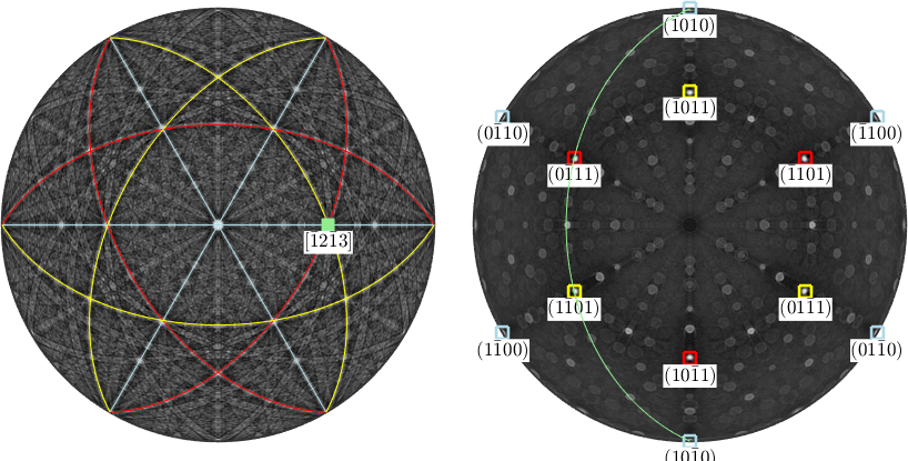

Note that MTEX automatically switches from reciprocal to direct coordinates for displaying the zone axis. The command round is required in order have the direction be scaled to integer Miller indices. Let us now consider a second crystal direction

d2 = Miller(-2,0,1,cs,'uvw')

plot(d2,'marker','s','parent',ax1,'MarkerFaceColor','Orange','labeled','backgroundColor','w')
circle(d2,'parent',ax2,'linecolor','orange')

d2 = Miller (alpha-quartz low)
   u  v  w
  -2  0  1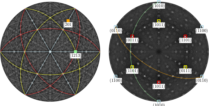

The two crystal directions d1 and d2 span a lattice plane which once again can be computed by the cross product of d1 and d2. In the Kikuchi pattern the lattice plane corresponds to the band connecting d1 and d2 where as in the dual Kikuchi pattern it coincides with the intersection of the two great circles representing d1 and d2.

n = round(cross(d1,d2))

circle(n,'parent',ax1,'linecolor','white')
plot(n,opt{:},'MarkerEdgeColor','white')

n = Miller (alpha-quartz low)
  h  k  i  l
  1 -2  1  2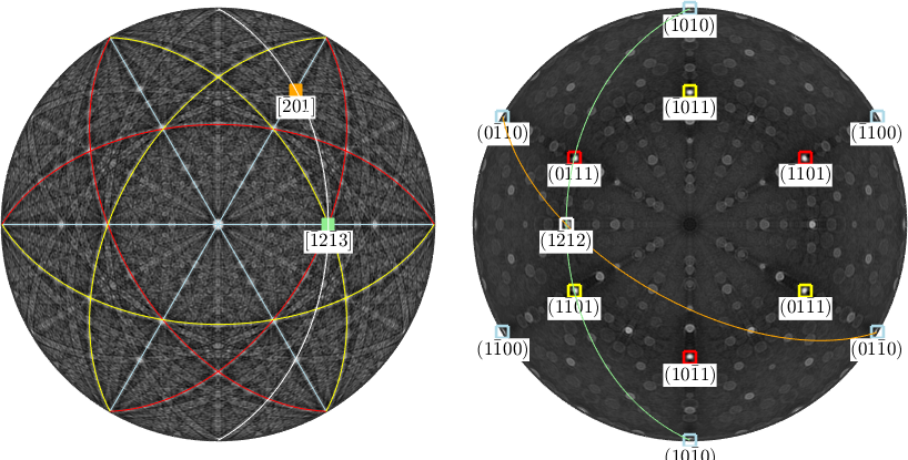

Angles

The angle between two crystal directions d1 and d2 is defined as the smallest angle between d1 and all symmetrically equivalent directions to d2. This angle is in radiant and it is calculated by the function angle(d1,d2)

angle(Miller(1,1,-2,0,cs),Miller(-1,-1,2,0,cs)) / degree

ans =
   60.0000

As always the keyword 'antipodal' adds antipodal symmetry to this computation

angle(Miller(1,1,-2,0,cs),Miller(-1,-1,2,0,cs),'antipodal') / degree

ans =
   1.2074e-06

In order to ignore the crystal symmetry, i.e., to compute the actual angle between two directions use the option 'noSymmetry'

angle(Miller(1,1,-2,0,cs),Miller(-1,-1,2,0,cs),'noSymmetry') / degree

ans =
  180.0000

This option is available for many other functions involving crystal directions and crystal orientations.

Crystal Orientations

Crystal orientations describe how the crystal lattice is aligned with respect to a specimen fixed reference frame. Consider the crystal orientation

ori = orientation.byEuler(10*degree,20*degree,30*degree,cs)

close all
plot(ori * pattern,'resolution',0.25*degree,'complete','upper')
mtexColorMap black2white

ori = orientation (alpha-quartz low → y↑→x)
 
  Bunge Euler angles in degree
  phi1  Phi phi2
    10   20   30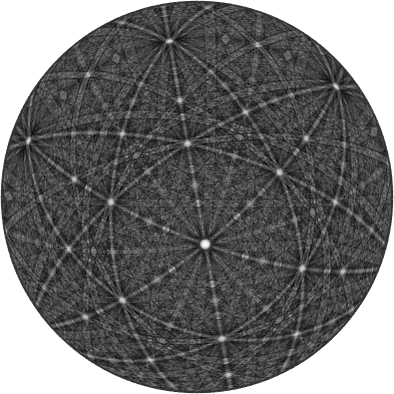

Then one can apply it to a crystal direction to find its coordinates with respect to the specimen coordinate system

ori * d1

hold on
plot(ori*d1,'marker','s','MarkerFaceColor','lightgreen','label',char(d1,'latex'),'backgroundColor','w')
hold off

ans = vector3d (y↑→x)
          x          y          z
  -0.427085 -0.0286108   0.592032

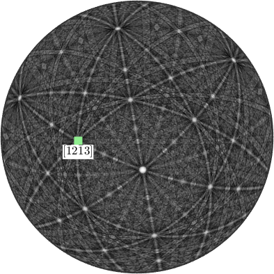
By applying a crystal symmetry one obtains the coordinates with respect to the specimen coordinate system of all crystallographically equivalent specimen directions.

hold on
plot(ori*d1.symmetrise ,'marker','s','MarkerFaceColor','lightgreen','label',char(d1,'latex'),'backgroundColor','w')
hold off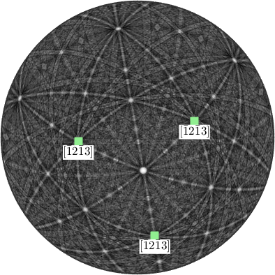

The above plot is essentially the pole figure representation of the orientation ori.

Conversions

Converting a crystal direction which is represented by its coordinates with respect to the crystal coordinate system \(a\), \(b\), \(c\) into a representation with respect to the associated Euclidean coordinate system is done by the command vector3d.

vector3d(d1)

ans = vector3d (y↑→x)
        x        y        z
  -0.2457 0.425565   0.5406

Conversion into spherical coordinates requires the function polar

[theta,rho] = polar(d1)

theta =
    0.7378
rho =
    2.0944