Embeddings of Orientations

Orientational embeddings are tensorial representations of orientations with the specific property that each class of symmetrically equivalent orientations has a unique tensor representation. The easiest tensorial representation of a rotation is its rotational matrix. However, in the presence of crystal symmetry multiple rotational matrices describe the same orientation. This can be avoided by restricting the space of admissible matrices to the so called fundamental region. However, this creates the problem that two similar orientations may be represented by very different matrices in the fundamental region. This usually happens if the orientations are close to the boundary of the fundamental region.

The central problem is that the geometry of the fundamental region is not the geometry of the orientation space. Lets demonstrate this by taking pairs \(\mathtt{ori_1}\), \(\mathtt{ori_2}\) of random orientations in the fundamental region

% consider cubic symmetry
cs = crystalSymmetry('432');

% random pairs of orientations in the fundamental sector
ori1 = project2FundamentalRegion(orientation.rand(100000,cs));
ori2 = project2FundamentalRegion(orientation.rand(100000,cs));

and compare their misorientation angle \(\omega(\mathtt{ori}_1,\mathtt{ori}_2)\) with the Euclidean distance \(\lVert \mathtt{tensor(ori_1)} - \mathtt{tensor(ori_2)} \rVert_2\) of the corresponding rotational matrices and the Euclidean distance \( \lVert \mathtt{R(ori_1)} - \mathtt{R(ori_2)} \rVert_2\) of the corresponding Rodrigues Frank vectors.

% compute the misorientation angles in degree
omega = angle(ori1,ori2)./degree;

% compute the Euclidean distance between the rotational matrices
distMat = norm(tensor(ori1) - tensor(ori2));

% compute the Euclidean distance between the Rodrigues Frank vectors
distRV = norm(Rodrigues(ori1) - Rodrigues(ori2));

% plot
figure('position',[200 200 1200 400 ])
subplot(1,3,1)
scatter(omega,distMat)
xlabel('\(\omega(\mathtt{ori}_1,\mathtt{ori}_2)\)','Interpreter','latex')
ylabel('\(|| \mathtt{tensor(ori_1)} - \mathtt{tensor(ori_2)}||_2\)','Interpreter','latex')

subplot(1,3,2)
scatter(omega,distRV)
xlabel('\(\omega(\mathtt{ori}_1,\mathtt{ori}_2)\)','Interpreter','latex')
ylabel('\(|| \mathtt{R(ori_1)} - \mathtt{R(ori_2)}||_2\)','Interpreter','latex')

subplot(1,3,3)
scatter(distMat,distRV)
xlabel('\(|| \mathtt{tensor(ori_1)} - \mathtt{tensor(ori_2)}||_2\)','Interpreter','latex')
ylabel('\(|| \mathtt{R(ori_1)} - \mathtt{R(ori_2)}||_2\)','Interpreter','latex')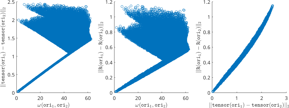

We observe that orientations with very small misorientation angle \(\omega(\mathtt{ori}_1,\mathtt{ori}_2)\) may be very far from each other in Rodrigues Frank space, i.e. \(\lVert\mathtt{R(ori_1)} - \mathtt{R(ori_2)}\rVert_2\) is large. As a consequence, we can not simply compute the average of two orientations by taking the mean of the corresponding Rodrigues vectors.

Lets have a look at an extremal case of finding the mean orientations of the orientations \((44^{\circ},0^{\circ},0^{\circ})\) and \((46^{\circ},0^{\circ},0^{\circ})\)

% define two orientations
ori = project2FundamentalRegion(orientation.byEuler([44 46]*degree,0,0,cs));

%compute the mean by averaging the Rodrigues vectors
mori = orientation.byRodrigues(mean(ori.Rodrigues),cs)

mori = rotation
 
  Bunge Euler angles in degree
  phi1  Phi phi2
     0    0    0

The mean orientation \((0^{\circ},0^{\circ},0^{\circ})\) computed from the average of the Rodrigues vectors is far away from the true mean.

mean(ori)

ans = orientation (432 → xyz)
 
  Bunge Euler angles in degree
  phi1  Phi phi2
    45    0    0

This issue does not only apply to the mean but actually to all statistical methods that work well for vectorial data and that one would like to apply to orientation data.

Defining an Embedding

The crucial idea of an embedding is to replace the vectorial representation by a higher dimensional tensorial representation that preserves the geometry and the distances of the orientation space as good as possible. In MTEX such an embedding \(\mathcal E(\mathtt{ori})\) of an orientation ori is defined by calling the function embedding.

e1 = embedding(ori1);
e2 = embedding(ori2)

e2 = embedding
 symmetry: 432
 ranks: 4
 dim: 9
 size: 100000 x 1

This creates variables e1 and e2 of type embedding that behaves like lists of vectors, i.e., they can be summed, rotated, scaled and one can compute their inner product. Lets have a look at the Euclidean distances \(\lVert\mathcal E(\mathtt{ori_1}) - \mathcal E(\mathtt{ori_2}) \rVert_2\) between the embeddings e1 and e2

% the Euclidean distance in the embedding
distE = norm(e1-e2) ./ degree;

close all
scatter(omega,distE)
xlabel('\(\omega(\mathtt{ori}_1,\mathtt{ori}_2)\)','Interpreter','latex')
ylabel('\(||\mathcal E(\mathtt{ori_1}) - \mathcal E(\mathtt{ori_2}) ||_2\)','Interpreter','latex')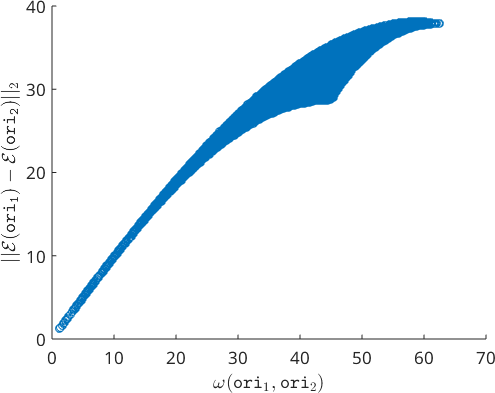

We observe that the distance in the embedding differs slightly from the misorientation angle. However, especially for small misorientation angles the approximation is very good.

Lets go back to our second example of averaging the orientations \((44^{\circ},0^{\circ},0^{\circ})\) and \((46^{\circ},0^{\circ},0^{\circ})\). If we compute the embedding of both orientations, average the resulting tensors and project the mean tensor back to an orientation we end up with the correct result \((45^{\circ},0^{\circ},0^{\circ})\).

% compute the embedding of the two orientations
e = embedding(ori);

% take the mean of the embeddings
me = mean(e);

% compute an orientation from the mean embedding
orientation(me)

ans = orientation (432 → xyz)
 
  Bunge Euler angles in degree
  phi1  Phi phi2
   315    0    0

Basic Properties

By construction the embeddings of all orientations have the same norm.

norm(embedding(orientation.rand(5,cs))).'

ans =
    0.3873    0.3873    0.3873    0.3873    0.3873

In other words the embeddings are located on the surface of a ball with a radius \(1\). When computing the mean from a list of embeddings the resulting tensor has in general a smaller norm, i.e., is inside this ball. Similarly as in spherical statistics the norm of the mean of the embeddings can be interpreted as a measure of the dispersion of the orientations. If the norm is close to 1 the orientations are tightly concentrated around a preferred orientation, whereas if the norm is close to zero some of the orientations are at maximum distance to each other.

Lets compare the norm

\[ n=\left\lVert\frac{1}{N} \sum_{i=1}^N \mathcal E(\mathtt{ori}_i) \right\rVert\]

of the mean embedding with the standard deviation

\[ \sigma = \left(\frac{1}{N} \sum_{i=1}^N \omega(\mathtt{ori}_i, \mathtt{mori})^2\right)^{1/2},\]

where \(\omega(\mathtt{ori}_i, \mathtt{mori})\) denotes the misorientation angle between the orientations \(\mathtt{ori}_i\) and the mean orientation \(\mathtt{mori}\).

% generate samples of orientations of different dispersion
n = []; sigma = [];
for hw = logspace(-1,1.75,40)*degree

  psi = SO3DeLaValleePoussinKernel('halfwidth',hw);
  odf = unimodalODF(orientation.rand(cs),psi);
  ori = discreteSample(odf,round(1000*(hw*6)^3));

  n(end+1) = norm(mean(embedding(ori)));

  sigma(end+1) = std(ori);
  progress(length(sigma),40);

end

plot(sigma,real(sqrt(1-n)),'linewidth',2)
xlabel('standard deviation \(\sigma\)','Interpreter','latex')
ylabel('\(\sqrt{1-n}\)','Interpreter','latex')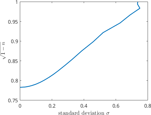

It appears as if the norm of the mean embedding is a function of the standard deviation. However, the reason for this false relationship is that we have generated the orientations out of a single family of random variables - unimodal de la Vallee Poussin distributed density functions. A broader family of density function are the Bingham distributions. Lets repeat the experiment for this family.

% genrate ODF of different halfwidth
n = []; sigma = [];
for k = 1:2:600

  kappa = rand(4,1);
  kappa = k * kappa ./sum(kappa);
  odf = BinghamODF(kappa,cs);
  ori = discreteSample(odf,1000);

  n(end+1) = norm(mean(embedding(ori)));
  sigma(end+1) = std(ori);

end

hold on
scatter(sigma,sqrt(1-n),'linewidth',2)
hold off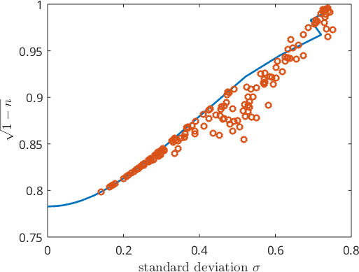

We observe that there is no one-to-one relationship between the discrete standard deviation.

Operations

The following operations are supported for embeddings:

Reference

The theory behind these embeddings is explained in the paper

%
%
%<html>
%   <div class="note">
%      <b>ok&lt;*SAGROW&gt;
%</b>
%      <text/>
%   </div>
%</html>
%