The curvature of a curve is defined by fitting locally a circle and taking one over its radius. Hence, a straight line will have curvature 0 and a circle of radius \(2\) will have constant curvature \(1/2\) everywhere. Hence, the unit of the curvature computed in MTEX is one over the unit of the EBSD coordinates which is usually 1/µm. Let us demonstrate boundary curvature use some artificial grain shapes
% import the artificial grain shapes
mtexdata testgrains silent

% select and smooth a few interesting grains
grains = smooth(grains('id',[2 3 9 11 15 16 18 23 31 33 38 40]),10);
Therefore, we first extract all boundary segments and colorize them according to their curvature.
% extract boundary segments
gB = grains.boundary;

% plot some dark background
plot(gB,'linewidth',10,'micronbar','off');

% colorize boundaries by curvature
hold on
plot(gB,gB.curvature,'linewidth',6);
hold off

% set a specific colormap
mtexColorMap('blue2red')
setColorRange(0.25*[-1,1])
mtexColorbar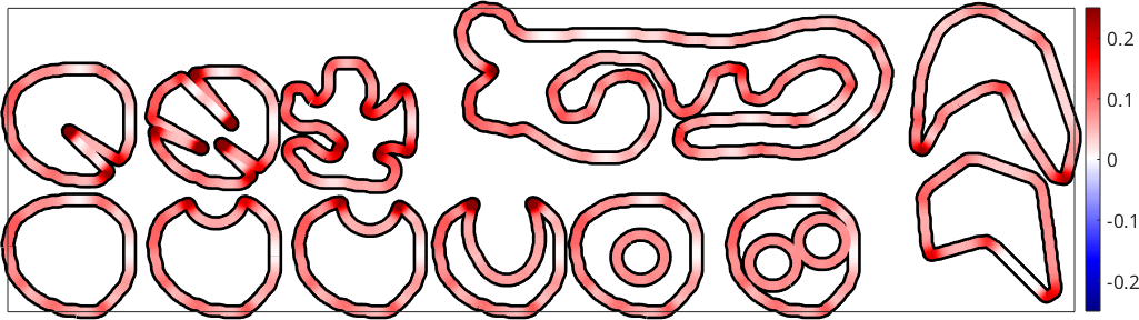
Note that all the curvature values are positive. This always happens if the curvature is computed for multiple grains at one. If we consider single grains and compute the curvature of single grain boundaries the sign of the values indicates whether the grain boundary is convex for concave with respect to the specific grain.
for k = 1:length(grains)

  gB = grains(k).boundary;
  plot(gB,'linewidth',10,'micronbar','off');
  hold on
  plot(gB,gB.curvature,'linewidth',6);

end
hold off

mtexColorMap('blue2red')
setColorRange(0.25*[-1,1])
drawNow(gcm,'figSize',getMTEXpref('figSize'))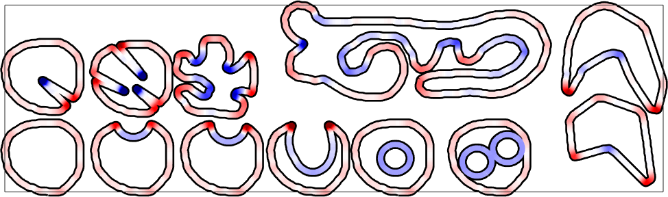
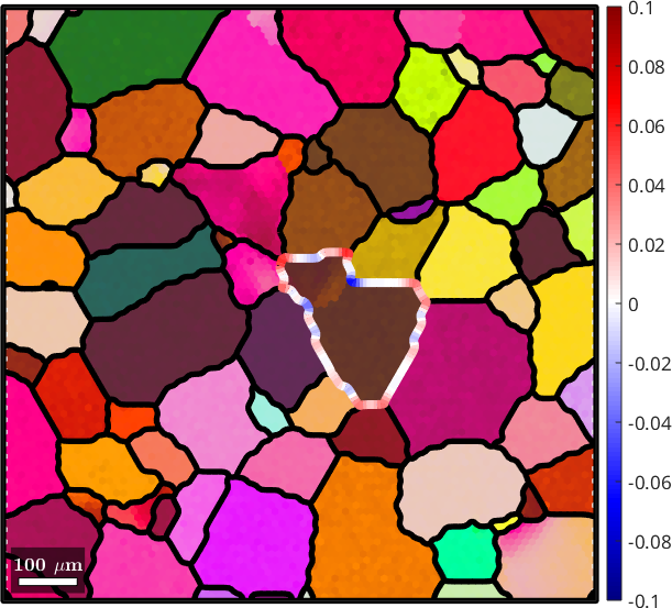
Finally we illustrate the usage of the curvature command at a real EBSD map.
% import data and reconstruct grains
mtexdata titanium silent
[grains,ebsd.grainId] = calcGrains(ebsd('indexed'));
grains = smooth(grains,5);

% plot an ipf map
plot(ebsd('indexed'),ebsd('indexed').orientations)

hold on

% plot grain boundaries
plot(grains.boundary,'linewidth',4)

% colorize the grain boundaries of grain 42 according to curvature
plot(grains(42).boundary,grains(42).boundary.curvature(5),'linewidth',6)
hold off
mtexColorMap('blue2red')
setColorRange(0.1*[-1,1])
mtexColorbar