Definition of Orientation Dependent Functions

Types of Orientation Dependent Functions

In MTEX any rotation / orientation dependent function is a variable of type SO3Fun. Internally, MTEX supports different types of representing such functions, e.g. by harmonic expansion or as superposition of kernel functions which are implemented as subclasses of the super class SO3Fun:

All representations allow for nearly the same operations. Furthermore, you can freely combine different representations within one expression. The most general representation is SO3FunHarmonic, i.e. every orientation dependent function S3F can be transformed into a harmonic series expansion using the syntax SO3FunHarmonic(S3F). That transformation is known as quadrature. Furthermore, many operations are only possible or significantly faster in the harmonic representation.

Additionally, MTEX supports orientation dependent vector fields by the class SO3VectorField.

In the following, we quickly show to set up the different types of orientation dependent functions.

By an explicit formula

Assume we have an explicit formula or algorithm to compute for an orientation a value. This could be the Taylor factor or any other physical property. Here we simply use the rotational angle. In order to a variable of type SO3Fun representing the rotational angle in degree we to do two steps.

Step 1: Define the relationship as an anonymous functions on SO(3)

The concept of anonymous functions in Matlab is explained here. In shorts it assigns a command / formula to a variable.

f = @(ori) angle(ori)./degree

f =
  function_handle with value:
    @(ori)angle(ori)./degree

Step 2: Define a variable of type SO3FunHandle

Next, we use the anonymous function to define a variable of type SO3FunHandle.

% define a crystal symmetry
cs = crystalSymmetry('cubic');

% define the SO3Fun
SO3F = SO3FunHandle(f,cs)

% visualize the function
plot(SO3F)

SO3F = SO3FunHandle (m-3m → xyz)
  eval: @(ori)angle(ori)./degree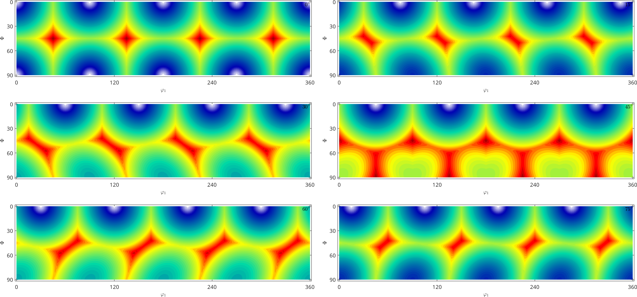

The plot shows the variation of the rotational angle with respect to the Euler angles under consideration of the crystal symmetry.

As Harmonic Expansion

As mentioned above we can translate any orientation dependent function into its harmonic series expansion. This is done by the command SO3FunHarmonic.

% transform SO3F into a harmonic series expansion
SO3F = SO3FunHarmonic(SO3F,'bandwidth',16)

% visualize the function
plot(SO3F)

SO3F = SO3FunHarmonic (m-3m → xyz)
  bandwidth: 16
  weight: 41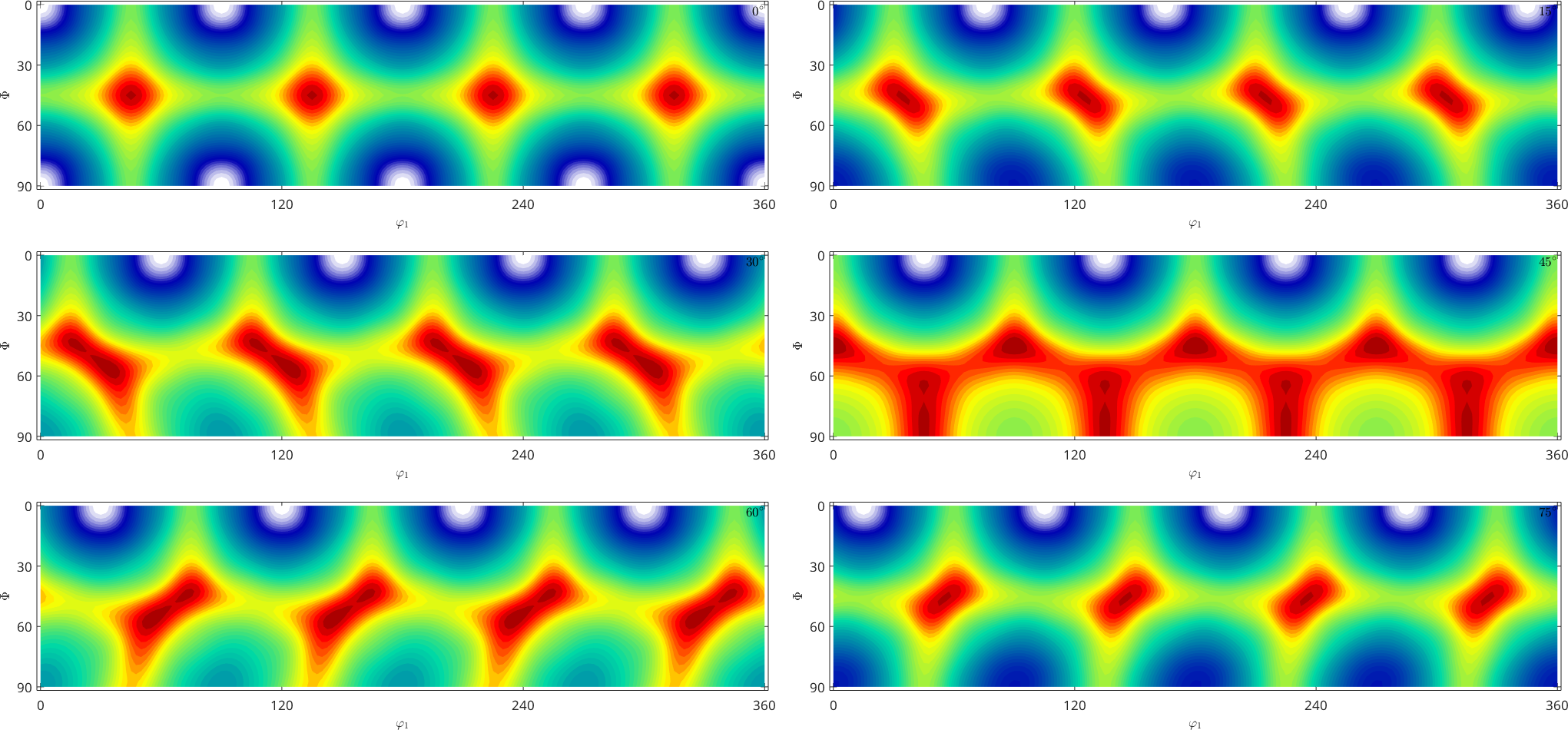

The difference to the previous plot is the cut off error due to the fixed bandwidth. Choosing a larger bandwidth would reduce the cut off error. Currently, a bandwidth of up to 128 works reasonably fast in MTEX. We may visualize the decay of the harmonic coefficients as follows

close all
plotSpektra(SO3F,'linewidth',2)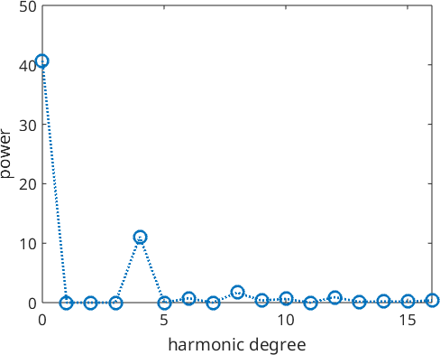

For further information on the Fourier coefficients, the bandwidth and other properties, see Harmonic Representation of Rotational Functions.

Superposition of Radial Functions

Radial functions are functions that depend only on the distance to some reference orientation. Typical examples are the de la Vallee Poussin kernel, the Abel Poisson kernel, the Gauss Weierstrass kernel or the von Mises Fisher kernel. The characterizing parameter of all these kernel functions is their halfwidth, i.e., the angular distance at which the function values is only half the function value at the center.

% define the kernel de la Vallee Poussin kernel with halfwidth 15 degree
psi = SO3DeLaValleePoussinKernel('halfwidth',15*degree)

close all
plot(psi)

psi = SO3DeLaValleePoussinKernel
  bandwidth: 17
  halfwidth: 15°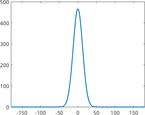

Using a large number of such kernel functions centered at different orientations allows to approximate arbitrary orientation dependent function. In MTEX superposition of radial functions naturally occur when performing ODF reconstruction from pole figure data or kernel density estimation from a small number of orientations, e.g.

% some random orientations
ori = orientation.rand(200,cs);

% perform kernel density estimation
SO3F = calcDensity(ori,'kernel',psi)

SO3F = SO3FunRBF (m-3m → xyz)
 
  multimodal components
  kernel: de la Vallee Poussin, halfwidth 15°
  center: 200 orientations

For further information see superposition of radial function.

Superposition of Fiber Elements

Similarly as with radial functions, we may also represent an orientation dependent function also as a superposition of fibre components. The typical case is that we want to model an fiber ODF. This can be done as follows

% define a fibre
f = fibre.beta(cs)

% define a density function along this fiber
SO3F = SO3FunCBF(f,'halfwidth',10*degree)

% plot it
plot(SO3F)

f = fibre (m-3m → xyz)
 
  h || r: (12 6 11) || (1,1,4)
 o1 → o2: (0°,35.3°,45°) → (90°,62.8°,45°)
 
SO3F = SO3FunCBF (m-3m → xyz)
 
  kernel: de la Vallee Poussin, halfwidth 10°
  fibre : (12 6 11) || 1,1,4
  weight: 1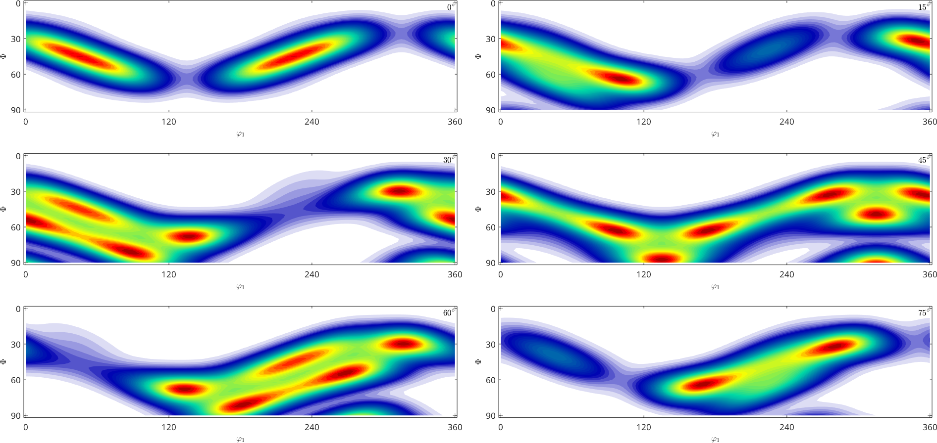

For further information, see fiber ODFs.

The Bingham Distribution

A last family of orientation dependent functions are Bingham distributions. Those are parameterized by a vector U of four orientations and a vector kappa of four values specifying the length and direction the half axes of a four dimensional ellipsoid.

kappa = [100 90 80 0];
U = [orientation.byAxisAngle(xvector,[0,180]*degree,cs),...
  orientation.byAxisAngle([yvector,zvector],180*degree,cs)]

SO3F = BinghamODF(kappa,U)

plot(SO3F)

U = orientation (m-3m → xyz)
  size: 1 x 4
 
  Bunge Euler angles in degree
  phi1  Phi phi2
     0    0    0
     0  180    0
    90  180  270
   180    0    0
 
 
SO3F = SO3FunBingham (m-3m → xyz)
 
  kappa: 100 90 80 0
  weight: 1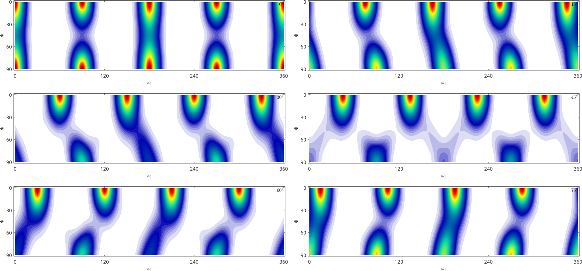

For further information, see SO3FunBingham.