On this page we consider the problem of determining a smooth orientation dependent function \(f(\mathtt{ori})\) given a list of orientations \(\mathtt{ori}_m\) and a list of corresponding values \(v_m\). These values may be the volume of crystals with a specific orientation, as in the case of an ODF, or any other orientation dependent physical property.
Orientation dependent data may be stored in ASCII files with lines of Euler angles, representing the orientations, and values. Such data files can be imported by the command orientation.load, where we have to specify the position of the columns of the Euler angles as well as of the additional properties.
fname = fullfile(mtexDataPath, 'orientation', 'dubna.csv');
[ori, S] = orientation.load(fname,'columnNames',{'phi1','Phi','phi2','values'});
As a result the command returns a list of orientations ori and a struct S. The struct contains one field for each additional column in our data file. In our toy example it is the field S.values. Lets generate a discrete plot of the given orientations ori together with the values S.values.
plotSection(ori, S.values,'all','sigma');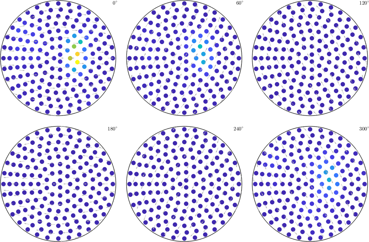
The process of finding a function which coincides with the given function values in the nodes reasonably well is called approximation (or interpolation). MTEX support different approximation schemes: approximation by harmonic expansion, approximation by radial functions and approximation by a Bingham distribution.
In MTEX we have the general command interp for any of this methods.
The Approximation by radial functions should be preferred, if:
- The underlying function is a density function, i.e. it is positive and has mean value 1 (use the flag 'density')
- Low/Medium number of nodes
The Approximation by harmonic expansion should be preferred, if:
- The underlying function describes some other orientation dependent relationship
- Lots of nodes, outliers and noise
But this are only hints. In practical applications we should try both methods and decide on the basis of computational costs and the results.
Approximation by Harmonic Expansion
An approximation by harmonic expansion is computed by the command interp with the flag 'harmonic'. Internally MTEX uses the SO3FunHarmonic.interpolate method here.
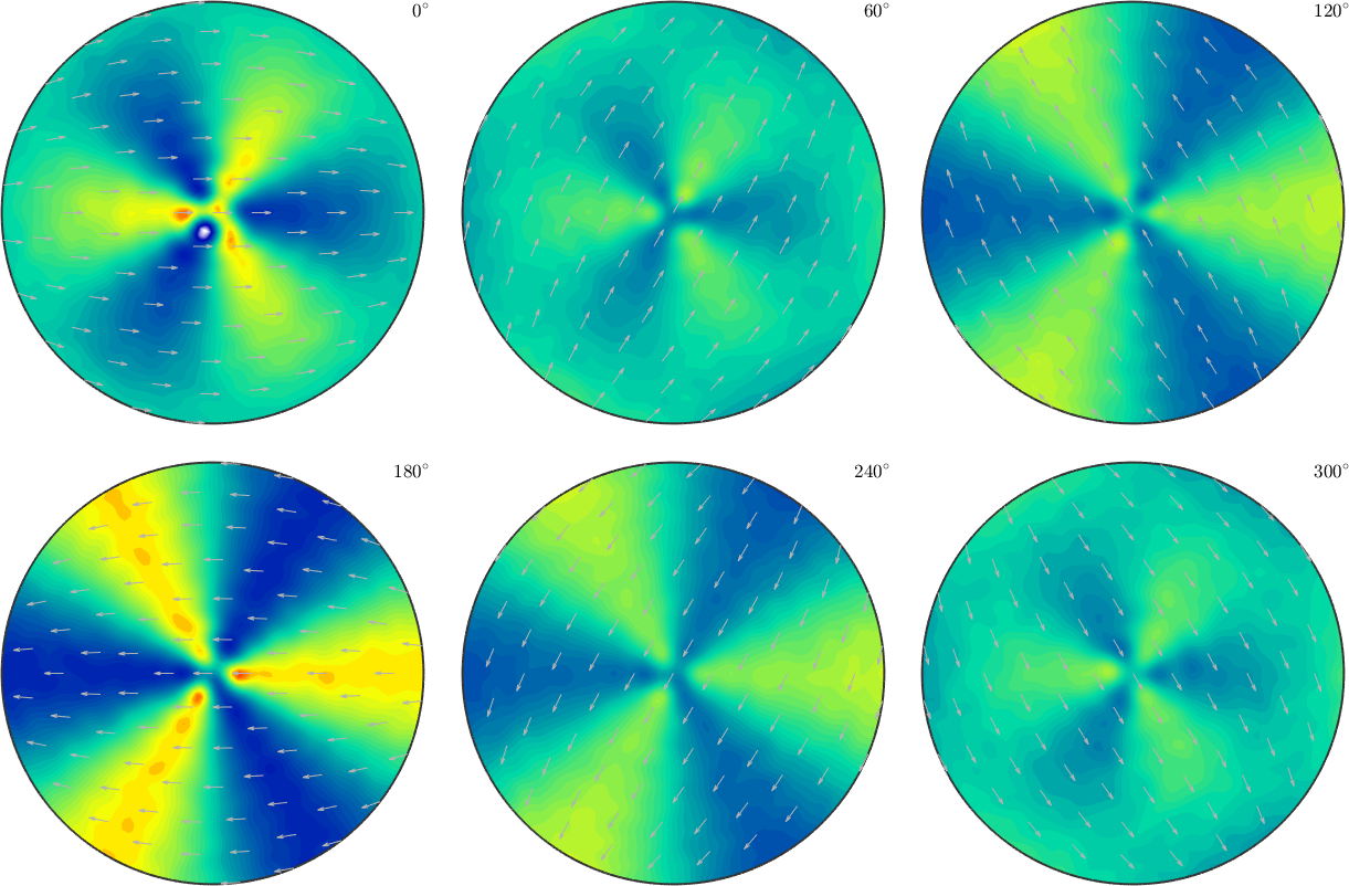
SO3F = interp(ori,S.values,'harmonic')
plot(SO3F,'sigma')
SO3F = SO3FunHarmonic (1 → y↑→x)
bandwidth: 18
weight: 0.98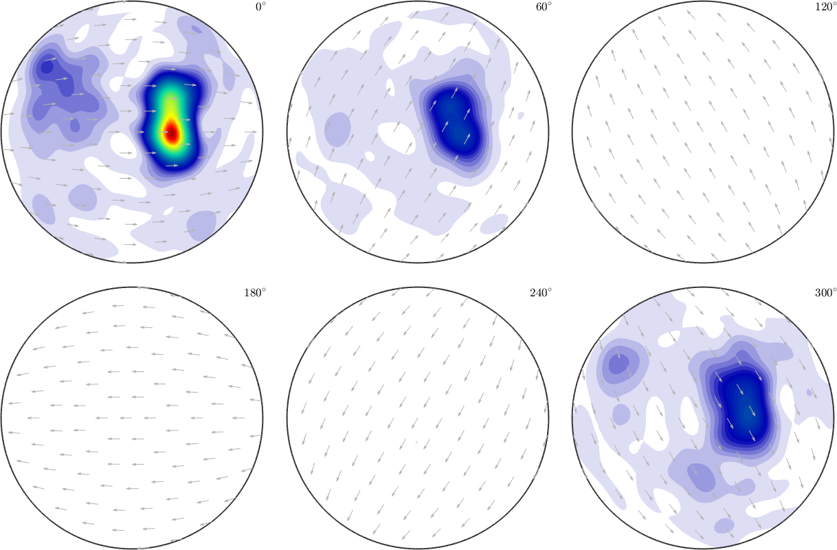
Note that SO3FunHarmonic.interpolate does not aim at replicating the values exactly. In fact the relative error between given data and the function approximation is
norm(SO3F.eval(ori) - S.values) / norm(S.values)ans =
0.0492The reason for this difference is that MTEX by default applies regularization. The default regularization parameter is \(\lambda = 10^{-8}\). We can switch off regularization by setting this value to \(0\).
SO3F = interp(ori,S.values,'harmonic','regularization',0)
% the relative error
norm(SO3F.eval(ori) - S.values) / norm(S.values)
plot(SO3F,'sigma')Warning: Maximum number of iterations reached, result may not have converged to
the optimum yet.
SO3F = SO3FunHarmonic (1 → y↑→x)
  bandwidth: 18
  weight: 0.98
ans =
0.0515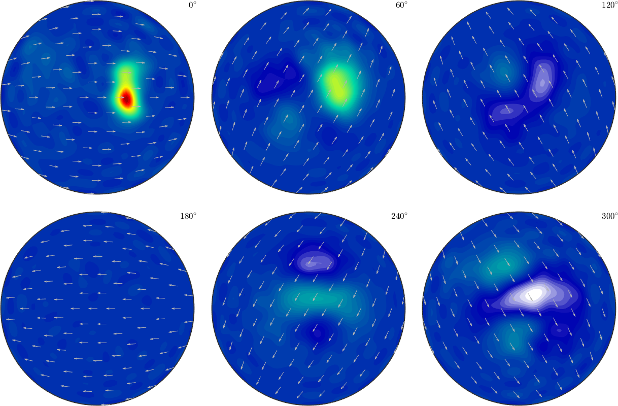
We observe that the relative error is much smaller, however the oscillatory behavior of the approximated function indicates overfitting. A more detailed discussion about choosing a good regularization parameter can be found in the section harmonic approximation theory.
An alternative way of regularization is to reduce the harmonic bandwidth
SO3F = interp(ori,S.values,'harmonic','regularization',0,'bandwidth',16)

% the relative error
norm(SO3F.eval(ori) - S.values) / norm(S.values)

plot(SO3F,'sigma')
SO3F = SO3FunHarmonic (1 → y↑→x)
bandwidth: 16
weight: 0.99
ans =
0.1064
One big disadvantage of harmonic approximation is that the resulting function is not guarantied to be non negative, even if all given function values have been non negative.
min(SO3F)ans =
-12.4261The possibility to guaranty non negativity is the central advantage of kernel based approximation.
Approximation by Radial Functions
The internal command for approximating orientation dependent data by a superposition of radial functions is SO3FunRBF.interpolate. Generally we can use the interp command.
SO3F = interp(ori,S.values,'density');

% the relative error
norm(SO3F.eval(ori) - S.values) / norm(S.values)

plot(SO3F,'sigma')
ans =
0.0125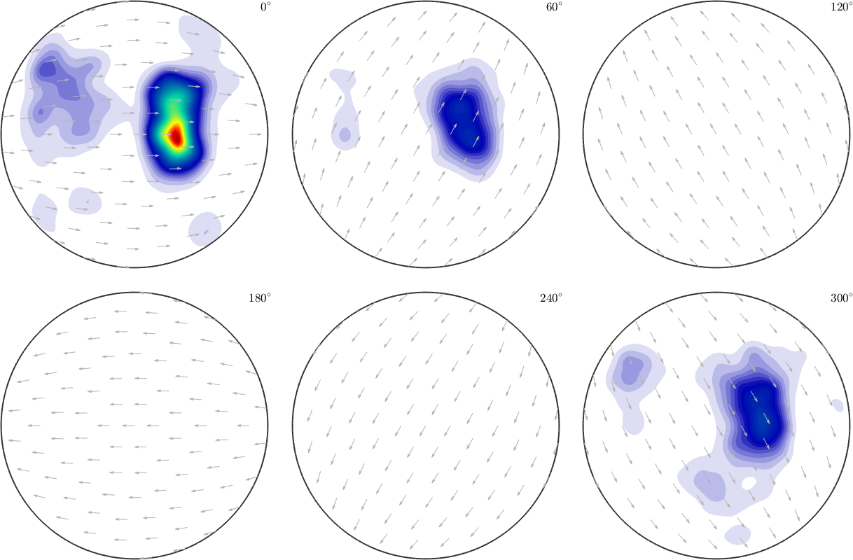
The option 'density' ensures that the resulting function is nonnegative and is normalized to \(1\).
minValue = min(SO3F)

meanValue = mean(SO3F)
minValue =
3.3899e-05
meanValue =
1The key parameter when approximation by radial functions is the halfwidth of the kernel function. This can be set by the option 'halfwidth'. A large halfwidth results in a very smooth approximating function whereas a very small halfwidth may result in overfitting
psi = SO3DeLaValleePoussinKernel('halfwidth',2.5*degree);
SO3F = interp(ori,S.values,'kernel',psi,'density');

plot(SO3F,'sigma')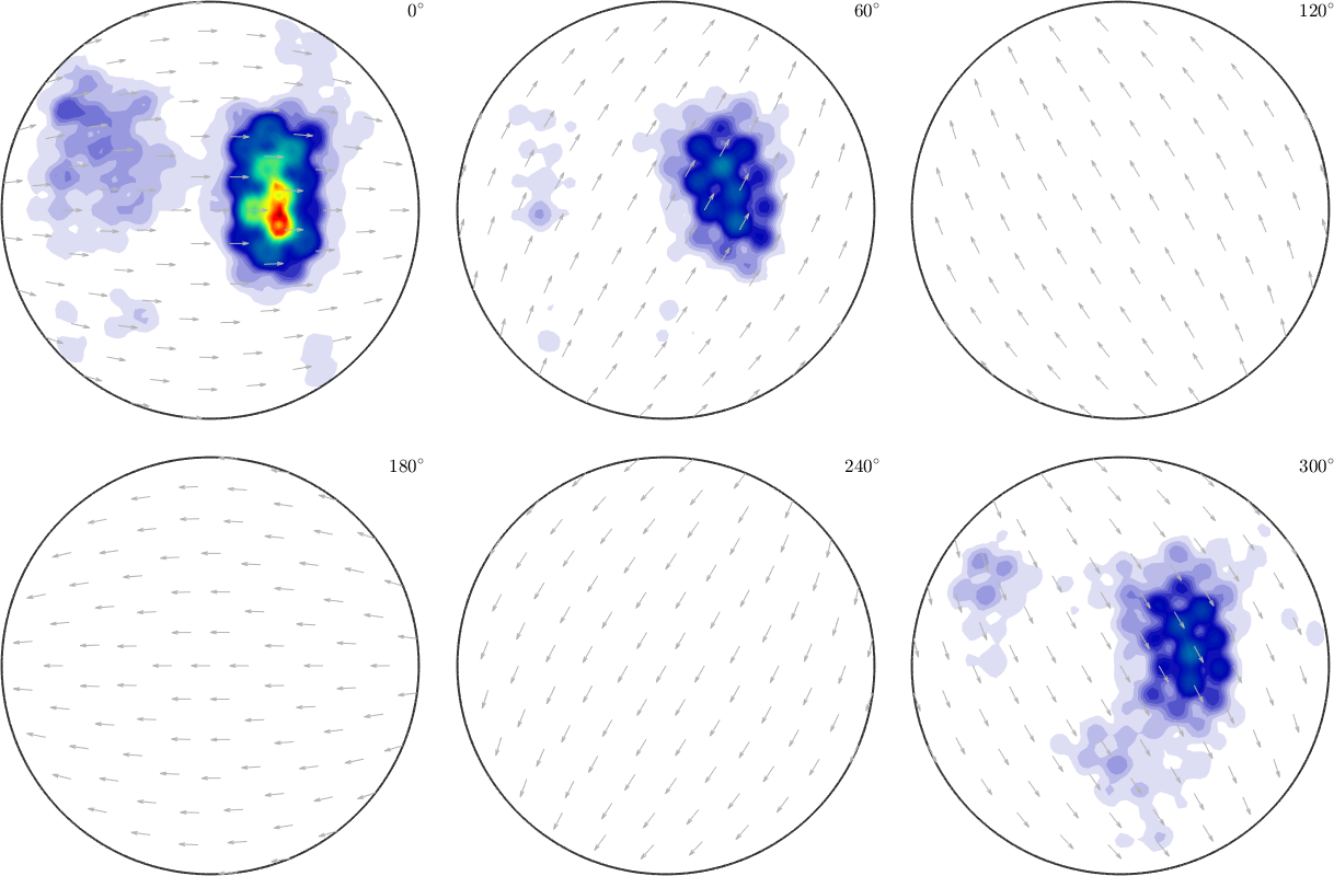
A more detailed discussion about the correct choice of the halfwidth and other options can be found in the section theory of RBF approximation.
If we omit the option 'density' the resulting function may have negative values similar to the harmonic setting
SO3F = interp(ori,S.values);

% the relative error
norm(SO3F.eval(ori) - S.values) / norm(S.values)

plot(SO3F,'sigma')
ans =
6.1048e-04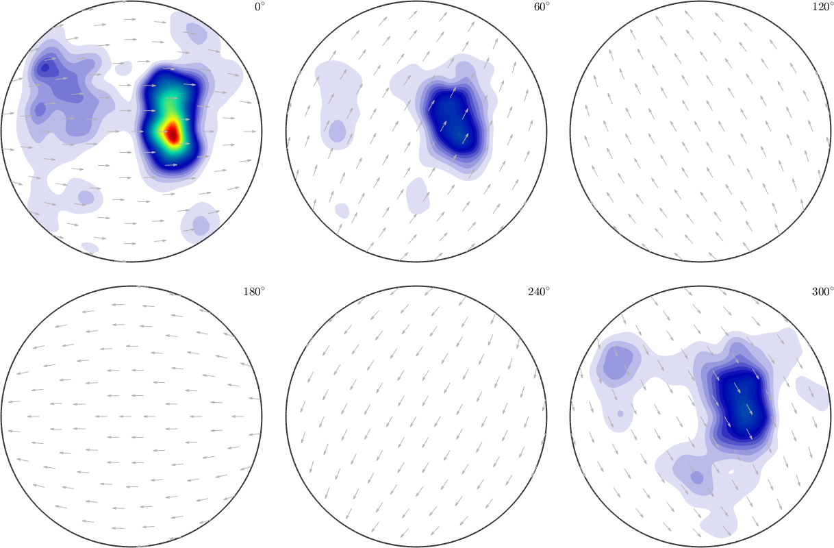
In general, omitting the option 'density' does not yield to a density function (nonnegative and mean 1).
minValue = min(SO3F)

meanValue = mean(SO3F)
minValue =
-6.0528
meanValue =
0.9806Approximation using the Bingham distribution
Approximation with the Bingham distribution currently works only with no symmetry.
TODO: Dont work
% simulate nodes and values from an odf
rng(0)
cs = crystalSymmetry("1");
odf = fibreODF(fibre.rand(cs));
S3G = equispacedSO3Grid(cs);
v = odf.eval(S3G);

% plot the underlying odf
figure(1)
plot(odf)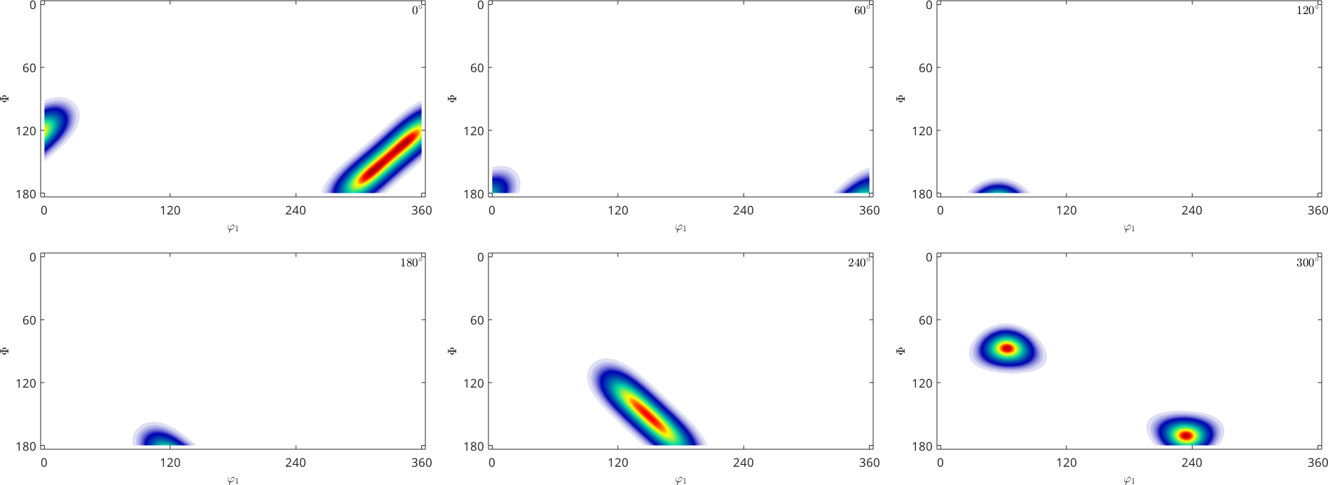
Now we try to approximate the Bingham distribution from the given orientations and there corresponding function values.
This is computed by the interp-command with the flag 'bingham'. Internally MTEX uses the SO3FunBingham.interpolate-method here.
SO3F = interp(S3G,v,'bingham')
% SO3F = SO3FunBingham.interpolate(S3G,v)

figure(2)
plot(SO3F)
SO3F = SO3FunBingham (1 → y↑→x)
kappa: 92 92 0 0
weight: 1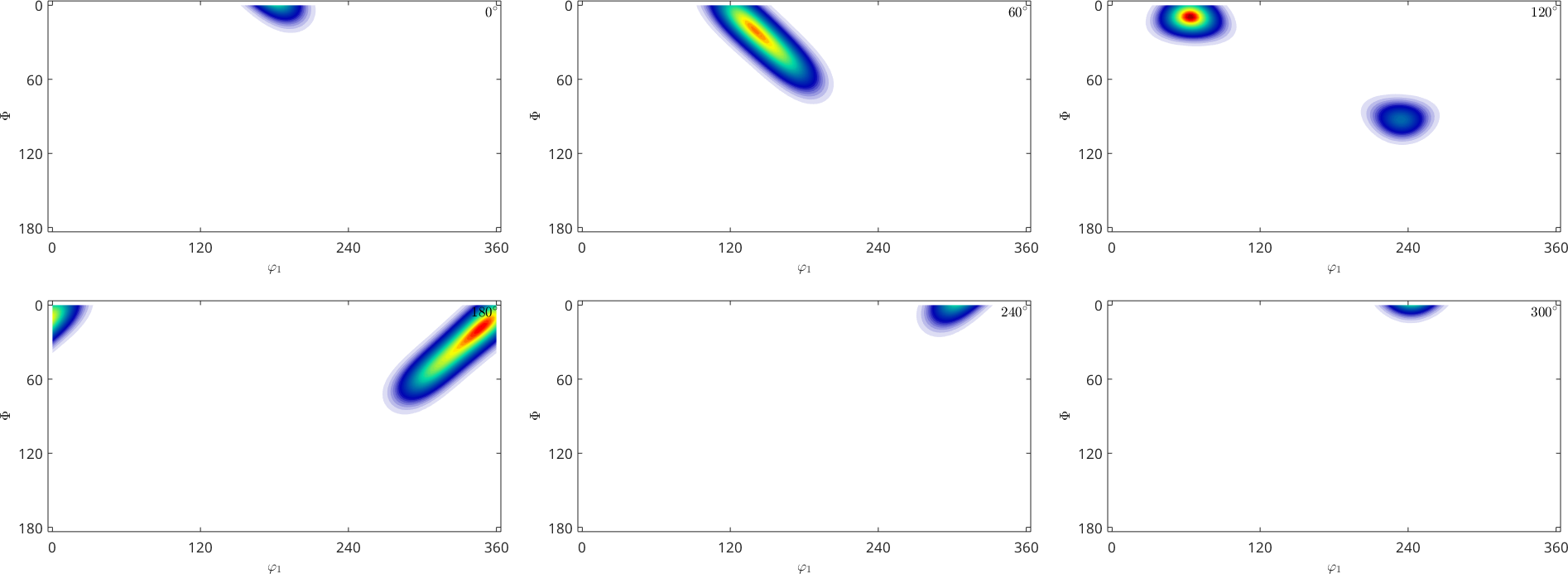
Alternative Non-ODF example
Lets consider an academic example which do not describe an underlying odf. Hence we have given noisy evaluations of the function
\[ f({\bf{R}}) = \cos(\omega({\bf{R}})) \cdot \sin(3\cdot \varphi_1({\bf{R}}))+\frac12 \]
in some random orientations, where \(\omega({\bf{R}})\) is the angle of the rotation \(\bf{R}\) and \(\varphi_1({\bf{R}})\) is the \(varphi_1\)-Euler angle of \(\bf{R}\).
f = SO3FunHandle(@(r) cos(r.angle).*sin(3*r.phi1) + 0.5);
plot(f,'sigma')

% random orientations and noisy evaluations
rng(0)
ori2 = orientation.rand(1e5);
val2 = f.eval(ori2);
val2 = val2 + randn(size(val2)) * 0.05 * std(val2);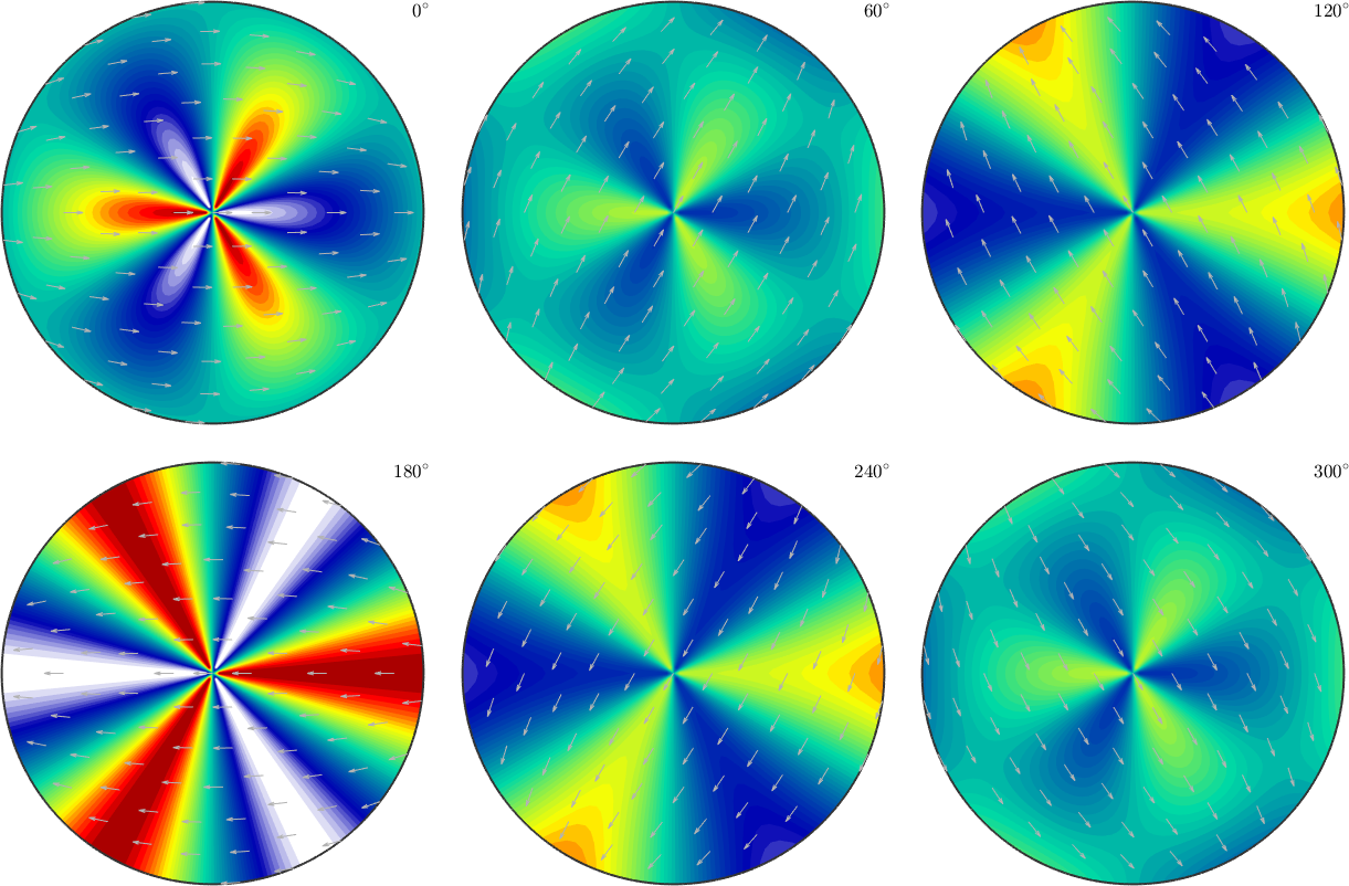
Lets compare the harmonic approximation and the RBF-Kernel approximation with respect to this example.
Harmonic Approximation
FH = interp(ori2, val2,'harmonic')
plot(FH,'sigma')
FH = SO3FunHarmonic (1 → y↑→x)
bandwidth: 40
weight: 0.5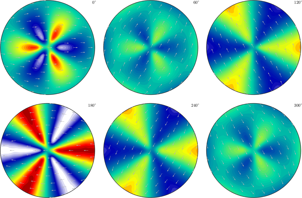
RBF-Kernel Approximation
FK = interp(ori2, val2)
plot(FK,'sigma')
FK = SO3FunRBF (1 → y↑→x)
multimodal components
kernel: de la Vallee Poussin, halfwidth 5°
center: 119088 orientations, resolution: 5°
weight: 0.5