Theory of Misorientations

Theory of Misorientations edit page

Misorientation describe the relative orientation of two crystal with respect to each other. Those crystal may be of the same phase or of different phases. Misorientation are used to describe orientation relationships at grain boundaries, orientation relationships during phase transformations or twinning and orientation gradients within grains.

Misorientations within the same phase

Misorientation describes the relative orientation of two grains with respect to each other. Important concepts are twinning and CSL (coincidence site lattice) misorientations. To illustrate this concept at a practical example let us first import some Magnesium EBSD data.

mtexdata twins silent

% use only proper symmetry operations
ebsd('M').CS = ebsd('M').CS.properGroup;

% compute grains
grains = calcGrains(ebsd('indexed'),'threshold',5*degree,'minPixel',5);
grains = smooth(grains,5);
CS = grains.CS; % extract crystal symmetry

Next we plot the grains together with their mean orientation and highlight grain 43 and grain 52

plot(grains,grains.meanOrientation,'micronbar','off')

hold on
plot(grains([43,52]).boundary,'edgecolor','w','linewidth',2)
hold off

text(grains([43,52]),{'1','2'})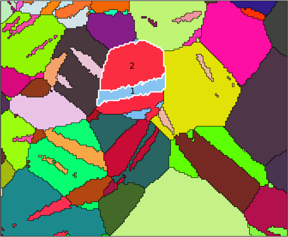

After extracting the mean orientation of grain 43 and 52

ori1 = grains(43).meanOrientation;
ori2 = grains(52).meanOrientation;

we may compute the misorientation angle between both orientations by

angle(ori1, ori2) ./ degree

ans =
   85.7299

Note that the misorientation angle is computed by default modulo crystal symmetry, i.e., the angle is always the smallest angles between all possible pairs of symmetrically equivalent orientations. In our example this means that symmetrisation of one orientation has no impact on the angle

angle(ori1, ori2.symmetrise) ./ degree

The misorientation angle neglecting crystal symmetry can be computed by

angle(ori1, ori2.symmetrise,'noSymmetry')./ degree

We see that the smallest angle indeed coincides with the angle computed before.

Misorientations

Remember that both orientations ori1 and ori2 map crystal coordinates onto specimen coordinates. Hence, the product of an inverse orientation with another orientation transfers crystal coordinates from one crystal reference frame into crystal coordinates with respect to another crystal reference frame. This transformation is called misorientation

mori = inv(ori1) * ori2

mori = misorientation (Magnesium → Magnesium)
 
  Bunge Euler angles in degree
     phi1     Phi    phi2
  149.583 94.2717 150.165

In the present case the misorientation describes the coordinate transform from the reference frame of grain 52 into the reference frame of crystal 43. Take as an example the plane $\{11\bar{2}0\}$ with respect to the grain 85. Then the plane in grain 43 which aligns parallel to this plane can be computed by

round(mori * Miller(1,1,-2,0,CS))

ans = Miller (Magnesium)
  h  k  i  l
  2 -1 -1  0

Conversely, the inverse of mori is the coordinate transform from crystal 43 to grain 52.

round(inv(mori) * Miller(2,-1,-1,0,CS))

ans = Miller (Magnesium)
  h  k  i  l
  1  1 -2  0

Coincident lattice planes

The coincidence between major lattice planes may suggest that the misorientation is a twinning misorientation. Lets analyze whether there are some more alignments between major lattice planes.

%m = Miller({1,-1,0,0},{1,1,-2,0},{1,-1,0,1},{0,0,0,1},CS);
m = Miller({1,-1,0,0},{1,1,-2,0},{-1,0,1,1},{0,0,0,1},CS);

% cycle through all major lattice planes
close all
for im = 1:length(m)
  % plot the lattice planes of grains 52 with respect to the
  % reference frame of grain 43
  plot(mori * m(im).symmetrise,'MarkerSize',10,...
    'DisplayName',char(m(im)),'figSize','large','noLabel','upper','textBelowMarker')
  hold on
end
hold off

% mark the corresponding lattice planes in the twin
mm = round(unique(mori*m.symmetrise,'noSymmetry'),'maxHKL',6);
annotate(mm,'labeled','MarkerSize',5,'figSize','large','textBelowMarker')

% show legend
legend({},'location','SouthEast','FontSize',13);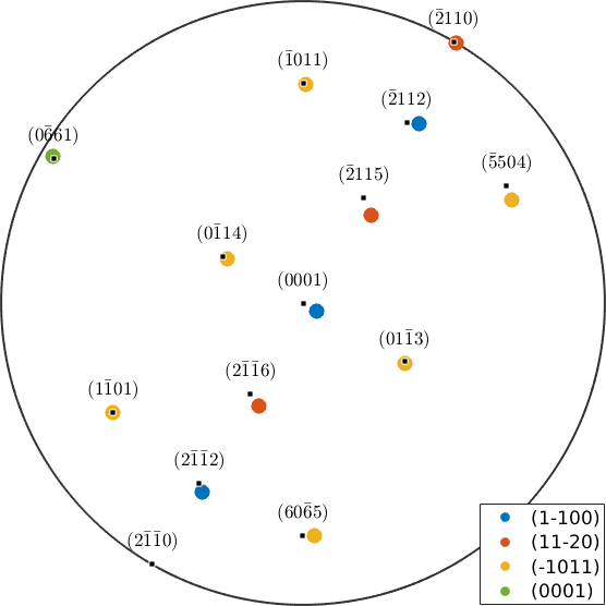

we observe an almost perfect match for the lattice planes $\{11\bar{2}0\}$ to $\{\bar{2}110\}$ and $\{1\bar{1}01\}$ to $\{\bar1101\}$ and good coincidences for the lattice plane $\{1\bar100\}$ to $\{0001\}$ and $\{0001\}$ to $\{0\bar661\}$. Lets compute the angles explicitly

angle(mori * Miller(1,1,-2,0,CS),Miller(2,-1,-1,0,CS)) / degree
angle(mori * Miller(1,0,-1,-1,CS),Miller(1,-1,0,1,CS)) / degree
angle(mori * Miller(0,0,0,1,CS) ,Miller(1,0,-1,0,CS),'noSymmetry') / degree
angle(mori * Miller(1,1,-2,2,CS),Miller(1,0,-1,0,CS)) / degree
angle(mori * Miller(1,0,-1,0,CS),Miller(1,1,-2,2,CS)) / degree

ans =
    0.4592
ans =
    0.1766
ans =
   59.6768
ans =
    2.6341
ans =
    2.5686

Twinning misorientations

Lets define a misorientation that makes a perfect fit between the $\{11\bar20\}$, $\{2\bar1\bar10\}$ lattice planes and the $[0001]$, $[01\bar10]$ lattice directions.

mori = orientation.map(Miller(1,1,-2,0,CS),Miller(2,-1,-1,0,CS),...
  Miller(0,0,0,1,CS,'uvw'),Miller(0,1,-1,0,CS,'uvw'))

% the rotational axis
round(mori.axis)

% the rotational angle
mori.angle / degree

mori = misorientation (Magnesium → Magnesium)
 
 (0001) || (01-10)   [1-100] || [0001]
 
 
ans = Miller (Magnesium)
  h  k  i  l
  1  1 -2  0
ans =
    90

and plot the same figure as before with the exact twinning misorientation.

% cycle through all major lattice planes
close all
for im = 1:length(m)
  % plot the lattice planes of grains 52 with respect to the
  % reference frame of grain 43
  plot(mori * m(im).symmetrise,'MarkerSize',10,...
    'DisplayName',char(m(im)),'figSize','large','noLabel','upper')
  hold on
end
hold off

% mark the corresponding lattice planes in the twin
mm = round(unique(mori*m.symmetrise,'noSymmetry'),'maxHKL',6);
annotate(mm,'labeled','MarkerSize',5,'figSize','large')

% show legend
legend({},'location','NorthWest','FontSize',13);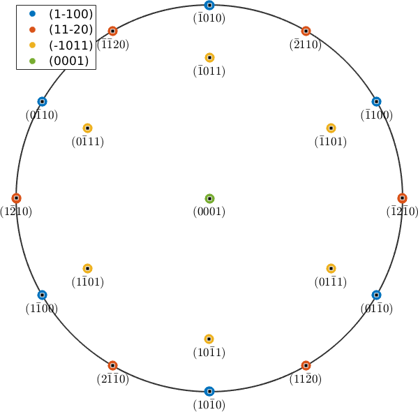

Highlight twinning boundaries

It turns out that in the previous EBSD map many grain boundaries have a misorientation close to the twinning misorientation we just defined. Lets Lets highlight those twinning boundaries

% consider only Magnesium to Magnesium grain boundaries
gB = grains.boundary('Mag','Mag');

% check for small deviation from the twinning misorientation
isTwinning = angle(gB.misorientation,mori) < 7.5*degree;

% plot the grains and highlight the twinning boundaries
plot(grains,grains.meanOrientation,'micronbar','off')
hold on
plot(gB(isTwinning),'edgecolor','w','linewidth',2)
hold off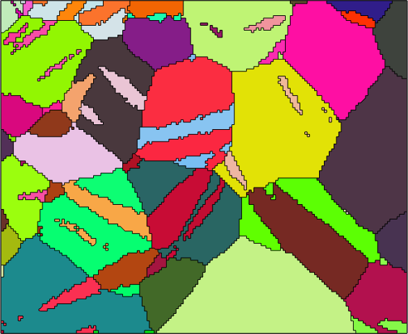

From this picture we see that large fraction of grain boundaries are twinning boundaries. To make this observation more evident we may plot the boundary misorientation angle distribution function. This is simply the angle distribution of all boundary misorientations and can be displayed with

close all
plotAngleDistribution(gB.misorientation)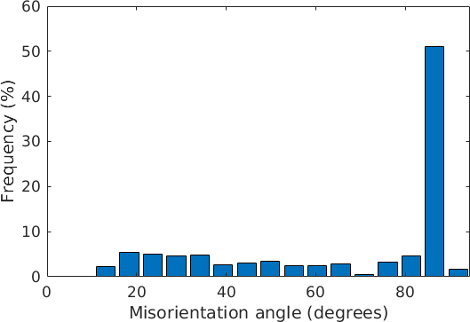

From this we observe that we have about 50 percent twinning boundaries. Analogously we may also plot the axis distribution

plotAxisDistribution(gB.misorientation,'contour')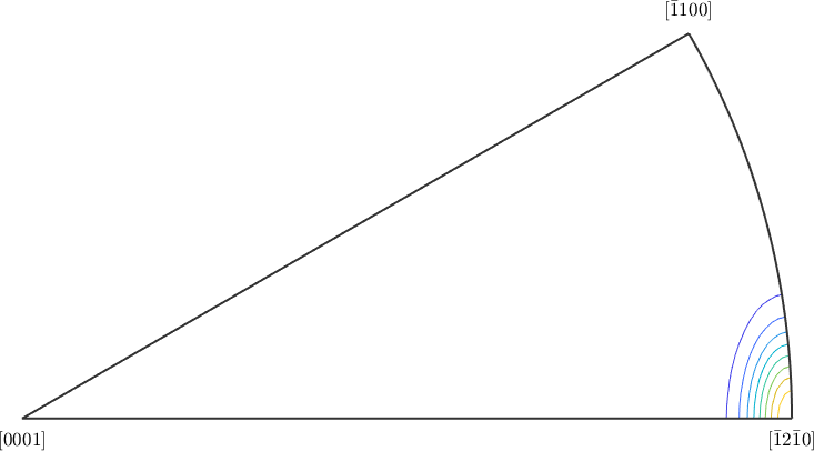

which emphasizes a strong portion of rotations about the $(\bar12\bar10)$ axis.

Phase transitions

Misorientations may not only be defined between crystal frames of the same phase. Lets consider the phases Magnetite and Hematite.

CS_Mag = loadCIF('Magnetite')
CS_Hem = loadCIF('Hematite')

CS_Mag = crystalSymmetry
 
  mineral : Magnetite    
  symmetry: m-3m         
  elements: 48           
  a, b, c : 8.4, 8.4, 8.4
 
 
CS_Hem = crystalSymmetry
 
  mineral        : Hematite          
  symmetry       : -3m1              
  elements       : 12                
  a, b, c        : 5, 5, 14          
  reference frame: X||a*, Y||b, Z||c*

The phase transition from Magnetite to Hematite is described in literature by $\{111\}_m$ parallel $\{0001\}_h$ and \{\bar101}_m$ parallel $\{10\bar10\}_h$. The corresponding misorientation is defined in MTEX by

Mag2Hem = orientation.map(...
  Miller(1,1,1,CS_Mag),Miller(0,0,0,1,CS_Hem),...
  Miller(-1,0,1,CS_Mag),Miller(1,0,-1,0,CS_Hem))

Mag2Hem = misorientation (Magnetite → Hematite)
 
 (01-1) || (0-110)   [111] || [0001]

Assume a Magnetite grain with orientation

ori_Mag = orientation.byEuler(0,0,0,CS_Mag)

ori_Mag = orientation (Magnetite → y↑→x)
 
  Bunge Euler angles in degree
  phi1  Phi phi2
     0    0    0

Then we can compute all variants of the phase transition by

symmetrise(ori_Mag) * inv(Mag2Hem)

ans = orientation (Hematite → y↑→x)
  size: 48 x 1

and the corresponding pole figures by

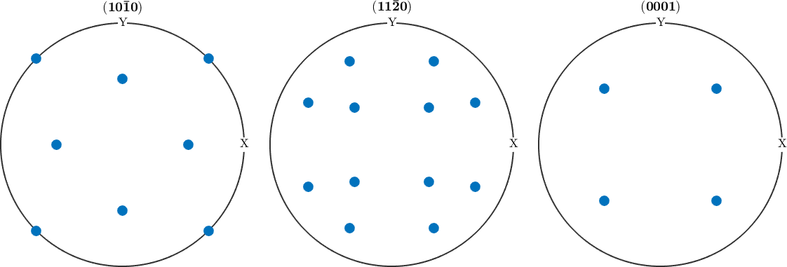
plotPDF(symmetrise(ori_Mag) * inv(Mag2Hem),...
  Miller({1,0,-1,0},{1,1,-2,0},{0,0,0,1},CS_Hem))