The linear theory of elasticity in anisotropic materials is essentially based on the fourth order stiffness tensor C. Such a tensor is represented in MTEX by a variable of type stiffnessTensor. Such a variable can either by set up using a symmetric 6x6 matrix or by importing it from an external file. The following examples does so for the stiffness tensor for Olivine
% file name
fname = fullfile(mtexDataPath,'tensor','Olivine1997PC.GPa');

% crystal symmetry
cs = crystalSymmetry('mmm',[4.7646 10.2296 5.9942],'mineral','Olivin');

% define the tensor
C = stiffnessTensor.load(fname,cs)
C = stiffnessTensor (Olivin)
unit: GPa
rank: 4 (3 x 3 x 3 x 3)
tensor in Voigt matrix representation:
320.5 68.2 71.6 0 0 0
68.2 196.5 76.8 0 0 0
71.6 76.8 233.5 0 0 0
0 0 0 64 0 0
0 0 0 0 77 0
0 0 0 0 0 78.7Hooke's Law
The stiffness tensor tensor of a material is defined as the stress the material experiences for a given strain
eps = strainTensor(diag([1,1.1,0.9]),cs)eps = strainTensor (Olivin)
type: Lagrange
rank: 2 (3 x 3)
1 0 0
0 1.1 0
0 0 0.9Now Hooke's law states that the resulting stress can be computed by
sigma = C : epssigma = stressTensor (Olivin)
rank: 2 (3 x 3)
459.9 0 0
0 353.4 0
0 0 366.2The other way the compliance tensor S = inv(C) translates stress into strain
inv(C) : sigmaans = strainTensor (Olivin)
type: Lagrange
rank: 2 (3 x 3)
1 0 0
0 1.1 0
0 0 0.9The elastic energy of the strain eps can be computed equivalently by the following equations
% the elastic energy
U = sigma : eps
U = EinsteinSum(C,[-1 -2 -3 -4],eps,[-1 -2],eps,[-3 -4]);

U = (C : eps) : eps;
U =
1.1783e+03Young's Modulus
Young's modulus is also known as the tensile modulus and measures the stiffness of elastic materials. It is computed for a specific direction d by the command YoungsModulus.
d = vector3d.X;
E = C.YoungsModulus(d)
E =
286.9284If the direction d is omitted Young's modulus is returned as a spherical function.
% compute Young's modulus as a directional dependent function
E = C.YoungsModulus

% which can be evaluated at any direction
E.eval(d)

% or plot it
setMTEXpref('defaultColorMap',blue2redColorMap);
plot(C.YoungsModulus,'complete','upper')
text([xvector,yvector,zvector],'labeled','BackgroundColor','w')
E = S2FunHarmonicSym (Olivin)
bandwidth: 128
antipodal: true
ans =
286.9284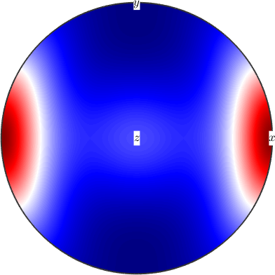
Linear Compressibility
The linear compressibility is the deformation of an arbitrarily shaped specimen caused by an increase in hydrostatic pressure and can be described by a second rank tensor. Similar to the Young's modulus it can be computed by the command linearCompressibility for specific directions d or as a spherical function
% compute as a spherical function
beta = linearCompressibility(C)

% plot it
plot(beta,'complete','upper')
text([xvector,yvector,zvector],'labeled','BackgroundColor','w')

% evaluate the function at a specific direction
beta.eval(d)
beta = S2FunHarmonicSym (Olivin)
bandwidth: 2
antipodal: true
ans =
0.0018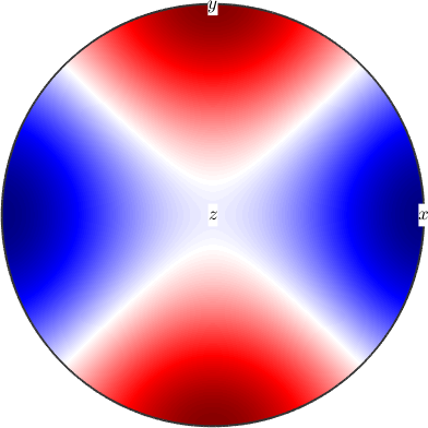
Poisson Ratio
The rate of compression / decompression in a direction n normal to the pulling direction p is called Poisson ratio.
% the pulling direction
p = vector3d.Z;

% two orthogonal directions
n = [vector3d.X,vector3d.Y];

% the Poisson ratio
nu = C.PoissonRatio(p,n)
nu =
0.1515 0.3383If we omit in the call to PoissonRatio the last argument
nu = C.PoissonRatio(p)nu = S2FunHarmonicSym (Olivin)
bandwidth: 4
antipodal: truewe again obtain a spherical function. However, this time it is only meaningful to evaluate this function at directions perpendicular to the pulling direction p. Hence, a good way to visualize this function is to plot it as a section in the x/y plane
plotSection(nu,p,'color','interp','linewidth',5)
axis off
mtexColorbar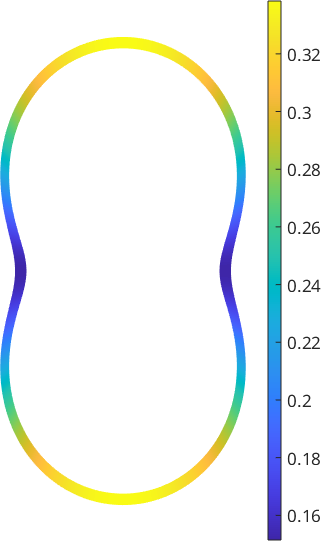
Shear Modulus
The shear modulus is TODO
% shear plane
n = Miller(0,0,1,cs);

% shear direction
d = Miller(1,0,0,cs);

G = C.shearModulus(n,d)
G =
6.2807e+04newMtexFigure('layout',[1,3])
% shear plane
n = Miller(1,0,0,cs);
plotSection(C.shearModulus(n),n,'color','interp','linewidth',5)
mtexTitle(char(n))
axis off
nextAxis
n = Miller(1,1,0,cs);
plotSection(C.shearModulus(n),n,'color','interp','linewidth',5)
mtexTitle(char(n))
nextAxis
n = Miller(1,1,1,cs)
plotSection(C.shearModulus(n),n,'color','interp','linewidth',5)
mtexTitle(char(n))
hold off
setColorRange('equal')
mtexColorbar
drawNow(gcm,'figSize','large')n = Miller (Olivin)
h k l
1 1 1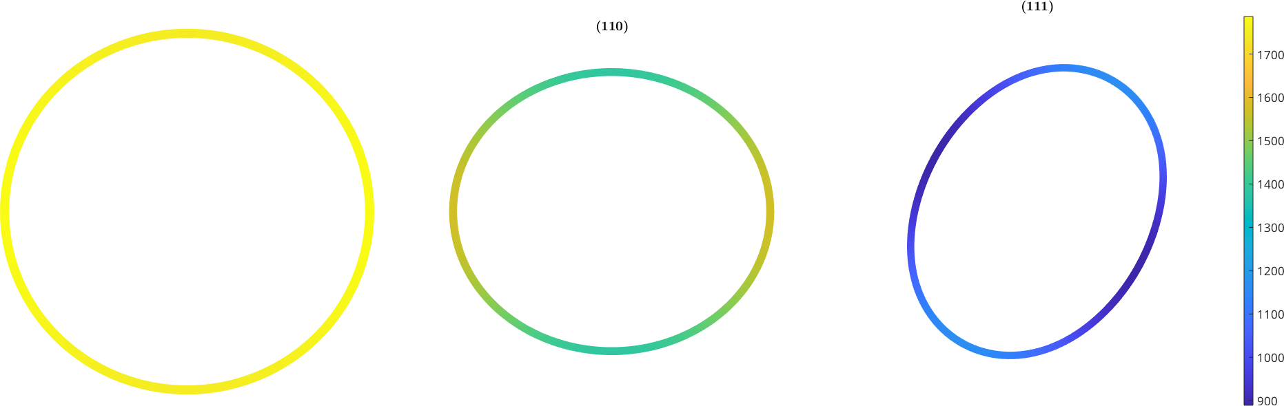
Wave Velocities
Since elastic compression and decompression is mechanics of waves traveling through a medium anisotropic compressibility causes also anisotropic waves speeds. The analysis of this anisotropy is explained in the section wave velocities.