By grain reconstruction we mean the subdivision of the specimen, or more precisely the measured surface of the specimen, into regions of similar orientation which we then call grains. Note that there is no canonical definition of what is a grain. The default grain reconstruction method in MTEX is based on the definition of high angle grain boundaries which are assumed at the perpendicular bisector between neighboring measurements whenever their misorientation angle exceeds a certain threshold. According to this point of view grains are regions surrounded by grain boundaries.
In order to illustrate the grain reconstruction process we consider the following sample data set
close all

% import the data
mtexdata forsterite

% restrict it to a subregion of interest.
ebsd = ebsd(inpolygon(ebsd,[5 2 10 5]*10^3));

% gridify the data
ebsd = ebsd.gridify;

% make a phase plot
plot(ebsd)
ebsd = EBSD (y↑→x)
Phase Orientations Mineral Color Symmetry Crystal reference frame
0 58485 (24%) notIndexed
1 152345 (62%) Forsterite LightSkyBlue mmm
2 26058 (11%) Enstatite DarkSeaGreen mmm
3 9064 (3.7%) Diopside Goldenrod 12/m1 X||a*, Y||b*, Z||c
Properties: bands, bc, bs, error, mad
Scan unit : um
X x Y x Z : [0, 36550] x [0, 16750] x [0, 0]
Normal vector: (0,0,1)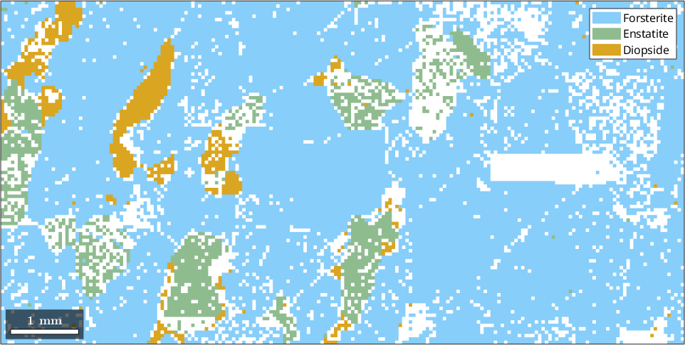
Basic grain reconstruction
We see that there are a lot of not indexed measurements. For grain reconstruction, we have three different choices how to deal with these unindexed regions:
- leave them unindexed
- assign them to the surrounding grains
- a mixture of both, e.g., assign small notindexed regions to the surrounding grains but keep large notindexed regions
The extent to which unindexed pixels are assigned is controlled by the parameter 'alpha'. Roughly speaking this parameter is the radius of the smallest unindexed region that will not be entirely assigned to surrounding grains. The default of this value is alpha = 2.2.
The second parameter 'angle' involved in grain reconstruction is the threshold misorientation angle indicating a grain boundary. By default, this value is set to angle = 10*degree.
Finally, the option 'minPixel' controls the minimum size of a reconstructed grain. Grains with less pixels are considered as not indexed.
All grain reconstruction methods in MTEX are accessible via the command calcGrains which takes as input an EBSD data set and returns a list of grain.
[grains, ebsd.grainId] = calcGrains(ebsd,'alpha',2.2,'angle',10*degree,'minPixel',5);
grains
grains = grain2d (y↑→x)
Phase Grains Pixels Mineral Symmetry Color
1 58 14017 Forsterite mmm LightSkyBlue
2 15 1375 Enstatite mmm DarkSeaGreen
3 21 693 Diopside 12/m1 Goldenrod
boundary segments: 3738 (171024 µm)
inner boundary segments: 1 (19 µm)
triple points: 112
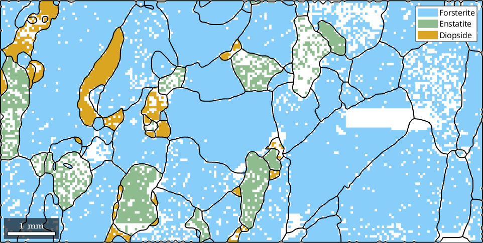
Properties: meanRotation, GOSThe reconstructed grains are stored in the variable grains. To visualize the grains we can plot its boundaries by the command plot.
% start override mode
hold on

% plot the boundary of all grains
plot(grains.boundary,'linewidth',1.5)

% stop override mode
hold off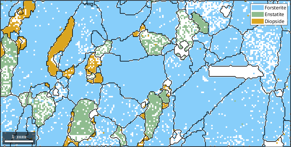
Grain Boundary Smoothing
Due to the gridded nature of the EBSD measurement the reconstructed grain boundaries often suffer from the staircase effect. This can be reduced by smoothing the grain boundaries using the command smooth
grains = smooth(grains,5);

% display the result
plot(ebsd)
hold on
plot(grains.boundary,'linewidth',1.5)
hold off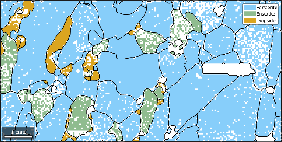
Adapting the Alpha Parameter
Increasing the parameter 'alpha' larger not indexed regions are associated to grains.
% reload the data
mtexdata forsterite silent
ebsd = ebsd(inpolygon(ebsd,[5 2 10 5]*10^3));
ebsd = ebsd.gridify;

[grains, ebsd.grainId] = calcGrains(ebsd,'alpha',10,'angle',10*degree,'minPixel',3);
grains = smooth(grains,5);

% plot the boundary of all grains
plot(ebsd)
hold on
plot(grains.boundary,'linewidth',1.5)
hold off