On this page we consider the problem of determining the Radial Basis Function (SO3FunRBF) of a smooth orientation dependent function \(f(\mathtt{ori})\) given a list of orientations \(\mathtt{ori}_m\) and a list of corresponding values \(v_m\). These values may be the volume of crystals with a specific orientation, as in the case of an ODF, or any other orientation dependent physical property.
A more general documentation about approximation of discrete data in MTEX can be found in the section Approximating Orientation Dependent Functions from Discrete Data.
In general we should favor RBF-kernel approximation, if the data coincide to an underlying density function (odf,mdf,...) or if the number of data points (given rotations and function values) and the noise ratio are not too large.
In the following we take a look on the approximation problem from general approximation theory, where we compared the harmonic approximation with kernel approximation.
Here we additionally assume that our function values are noisy.
fname = fullfile(mtexDataPath, 'orientation', 'dubna.csv');
[ori, S] = orientation.load(fname,'columnNames',{'phi1','Phi','phi2','values'});

val = S.values + randn(size(S.values)) * 0.2 * std(S.values);

plotSection(ori,val,'all','sigma')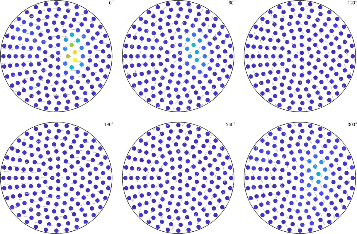
The basic strategy is to approximate the data by a SO3FunRBF, see Radial Basis Functions on SO(3).
Hence we determine rotations \(R_1,\dots,R_N\) and seek the corresponding coefficients \(\vec c=(c_1,\dots,c_N)\) such that
\[ f(x) = \sum_{n=1}^N c_n \, \Psi(\cos\frac{\omega(x,R_n)}{2}) \]
approximates our data reasonable well. In this formula, \(\Psi\) describes a SO(3)-Kernel Function. Hence, \(f\) is a superposition of one rotational kernel function centered on the orientations \(R_1,\dots,R_N\) and weighted by the coefficients \(c_1,\dots,c_N\).
A basic strategy is to apply least squares approximation, where we compute the coefficients \(c_n\) by minimizing the functional
\[ \sum_{m=1}^M|f(x_m)-v_m|^2 \]
for the given data points \((x_m,v_m)\), \(m=1,\dots,M\). Here \(x_m\) denotes the given orientations and \(v_m\) the corresponding function values.
This least squares problem can also be written in matrix vector notation \( \mathrm{argmin}\limits_{c} \| K \cdot c - v \|, \) where \(c=(c_1,\dots,c_N)^T\), \(v=(v_1,\dots,v_M)^T\) and \(K\) is the kernel matrix \([\Psi(\cos\frac{\omega(x_m,R_n)}{2})]_{m,n}\).
This least squares problem can be solved by the lsqr method from MATLAB, which efficiently seeks for roots of the derivative of the given functional (also known as normal equation).
Alternatively there is also a modified least square method mlsq, which search for a solution \(c_1,\dots,c_N\) that satisfies \(c>0\) and \(\sum\limits_{n=1}^N c_n = 1\). This method can be used if the underlying function is a density, i.e. it is nonnegative and has mean 1.
In MTEX the command interp computes by default computes an approximation by a superposition of radial functions.
SO3F = interp(ori,val,'density')
plot(SO3F,'sigma')
mtexColorbar
SO3F = SO3FunRBF (1 → y↑→x)
multimodal components
kernel: de la Vallee Poussin, halfwidth 5°
center: 72018 orientations, resolution: 5°
weight: 1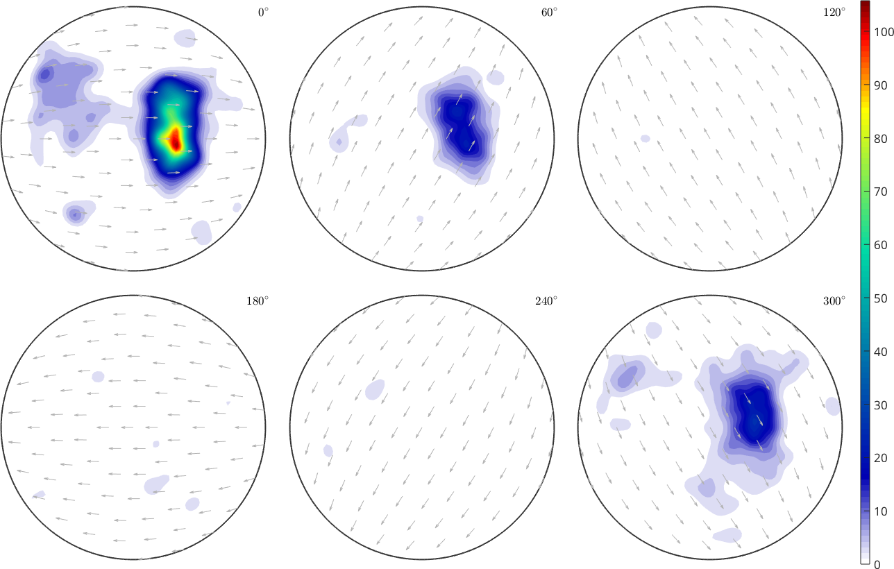
The flag 'density' tells MTEX to use the mlsq solver, which ensures that the resulting function is nonnegative and normalized to mean \(1\). This yields also a denoising effect.
minValue = min(SO3F)
meanValue = mean(SO3F)minValue =
1.1635e-06
meanValue =
1.0000One has to keep in mind that we can not expect the error in the data nodes to be zero, because we compute a smooth function from the noisy input data.
norm(SO3F.eval(ori) - val) / norm(val)ans =
0.1639In contrast, if we do not tell MTEX, that we try to approximate a density function, the solver has less information and the result is not denoised.
SO3F = interp(ori,val)
plot(SO3F,'sigma')
mtexColorbarSO3F = SO3FunRBF (1 → y↑→x)
multimodal components
kernel: de la Vallee Poussin, halfwidth 5°
center: 119088 orientations, resolution: 5°
weight: 0.95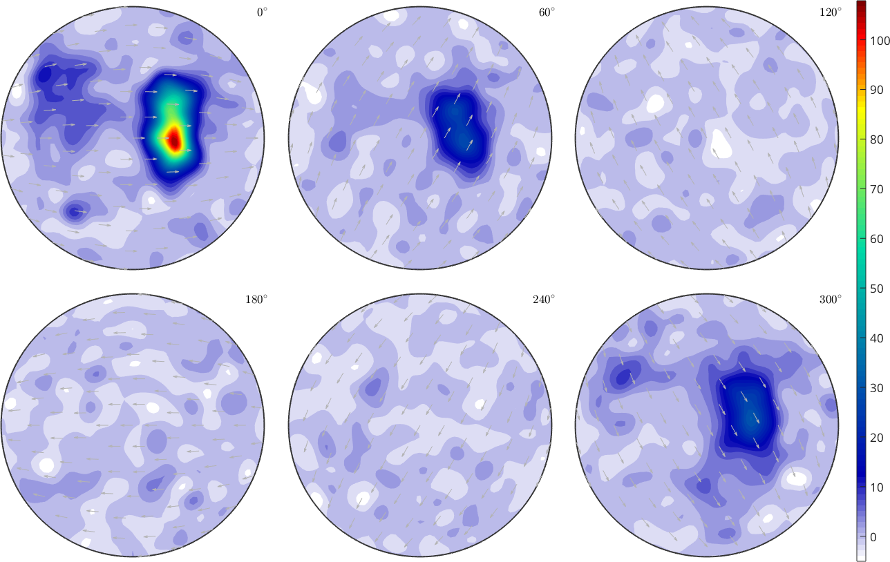
Hence the result is not automatically a density function (nonnegative and mean 1).
minValue = min(SO3F)
meanValue = mean(SO3F)minValue =
-6.7665
meanValue =
0.9518But since it is not denoised, it is overfitted and the error becomes small.
norm(SO3F.eval(ori) - val) / norm(val)ans =
4.7854e-04Adjustment of the Kernel Function
The key parameter when approximating by radial basis functions is the halfwidth of the kernel function \(\Psi\). This can be set by the option 'halfwidth'. A large halfwidth results in a very smooth approximated function whereas a very small halfwidth - in relation to the grid of the input data - may result in overfitting.
SO3F = interp(ori,val,'halfwidth',2*degree,'density')
plot(SO3F,'sigma')SO3F = SO3FunRBF (1 → y↑→x)
multimodal components
kernel: de la Vallee Poussin, halfwidth 2°
center: 1852941 orientations, resolution: 2°
weight: 1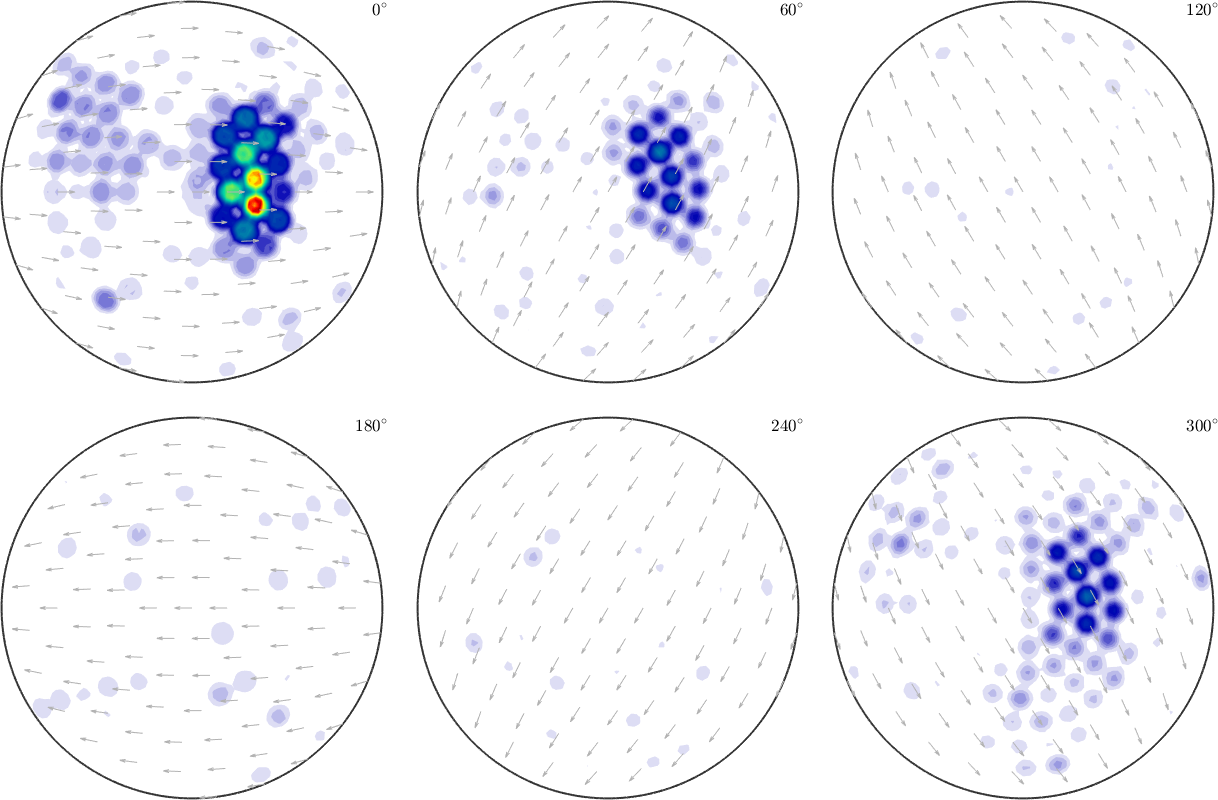
A a rule of thumb the halfwidth of the kernel function should be at least the resolution of the data points. Note that the option 'halfwidth' also adjusts the resolution of the center orientation grid of the rotational kernel functions of the approximated SO3FunRBF, i.e. the resolution of the grid of \(R_1,\dots,R_N\) in the above formulas.
We can preserve the resolution of this grid by adding the option 'resolution'. Therefore we obtain a smoothed function of SO3F1.
SO3F = interp(ori,val,'halfwidth',10*degree,'resolution',5*degree,'density')
plot(SO3F,'sigma')SO3F = SO3FunRBF (1 → y↑→x)
multimodal components
kernel: de la Vallee Poussin, halfwidth 10°
center: 70038 orientations, resolution: 5°
weight: 1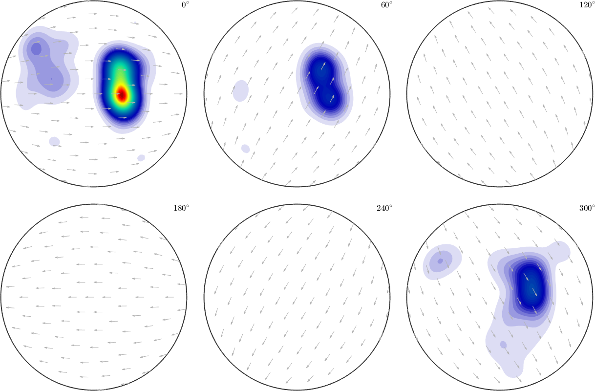
We can also input centers \(R_1,\dots,R_N\) for the rotational kernel functions by the option 'SO3Grid'.
S3G = equispacedSO3Grid(crystalSymmetry,'resolution',5*degree)
SO3F = interp(ori,val,'SO3Grid',S3G,'density')
plot(SO3F,'sigma')S3G = SO3Grid (1 → y↑→x)
grid: 119088 orientations, resolution: 5°
SO3F = SO3FunRBF (1 → y↑→x)

  multimodal components
  kernel: de la Vallee Poussin, halfwidth 5°
  center: 72018 orientations, resolution: 5°
  weight: 1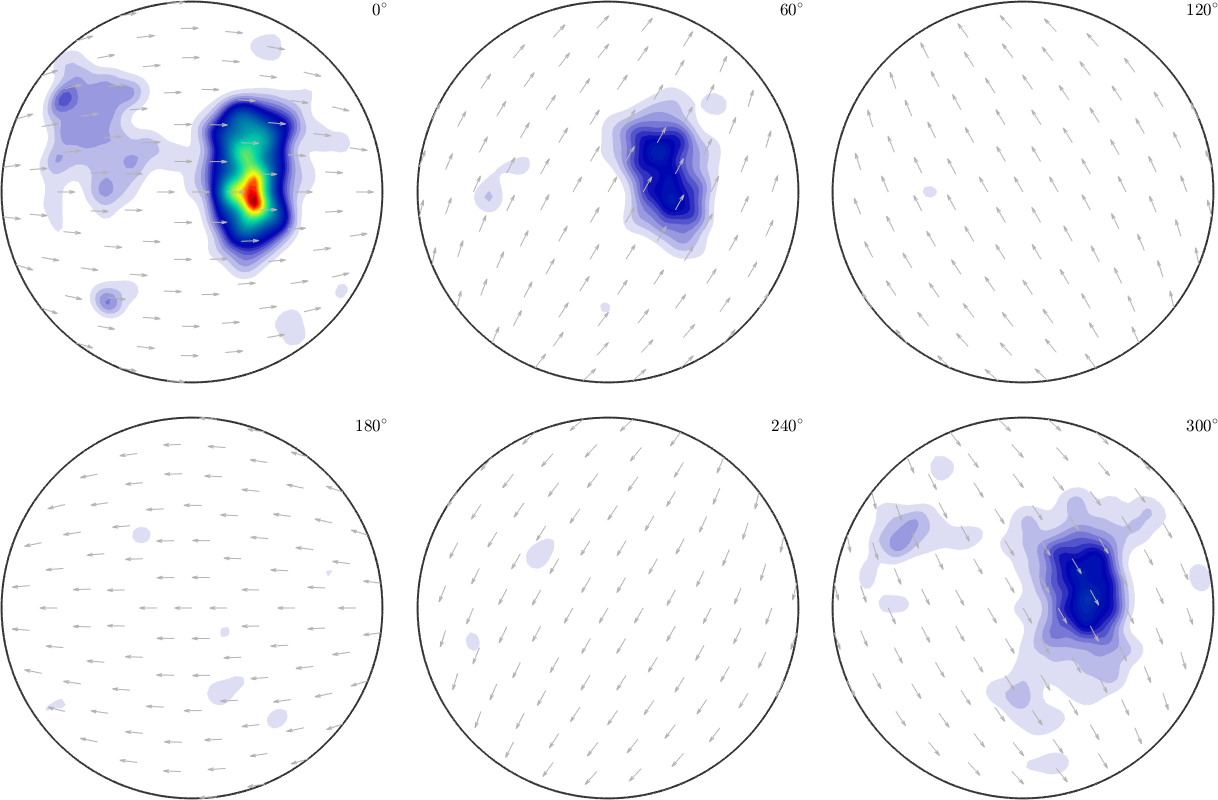
Lets study the effect of adjusting the kernel halfwidth to the error.
hw = [20,15,12.5,10,7.5,5,2.5];
err = zeros(size(hw));
for k = 1:numel(hw)
  SO3Fhw = interp(ori,val,'halfwidth',hw(k)*degree,'density');
  err(k) = norm(SO3Fhw.eval(ori) - S.values) / norm(S.values);
end

close all
plot(hw,err,'o--')
set(gca,'xdir','reverse')
xlabel('halfwidth [deg]')
ylabel('relative error')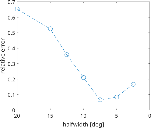
We may find the best fit with a halfwidth of 7.5°. If the system is underdetermined using a too small halfwidth, we may not be able to fit kernel weights without additional assumptions about the smoothness of the data.
SO3F = interp(ori,val,'halfwidth',7.5*degree,'density')
plot(SO3F,'sigma')
SO3F = SO3FunRBF (1 → y↑→x)
multimodal components
kernel: de la Vallee Poussin, halfwidth 7.5°
center: 24649 orientations, resolution: 7.5°
weight: 1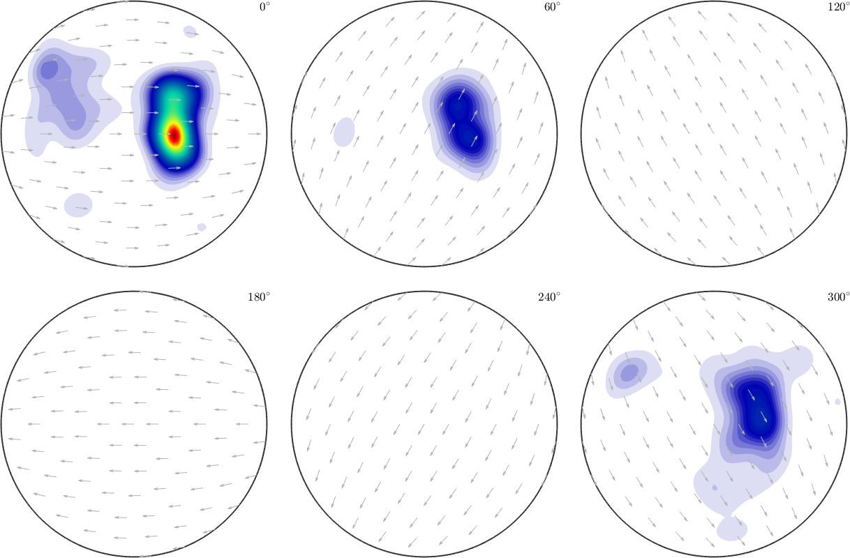
Note that the option 'halfwidth' tells MTEX to use the SO3DeLaValleePoussinKernel of this specific halfwidth. But we can also choose a different rotational kernel function by the option 'kernel'.
psi = SO3AbelPoissonKernel('halfwidth',5*degree)
SO3F = interp(ori,val,'kernel',psi,'density')
plot(SO3F,'sigma')
psi = SO3AbelPoissonKernel
bandwidth: 48
halfwidth: 5°
SO3F = SO3FunRBF (1 → y↑→x)
multimodal components
kernel: Abel Poisson, halfwidth 5°
center: 3989 orientations, resolution: 5°
weight: 1
Exact Interpolation
Assume, that our function values are not noisy. Then we may want to do exact interpolation, i.e. we want the error to be almost 0.
Up to now we used a special rotational grid for the centers of rotational kernel function the approximated SO3FunRBF. Now we can add the flag 'exact' to use the input nodes as centers for the rotational kernel functions. Therefore the kernel matrix \(K\) becomes symmetric, positive definite and the above linear system \(K\cdot c=v\) has a solution, i.e the error in lsqr may becomes 0. The disadvantage is that the kernel matrix is no longer sparse. Hence the computational costs may explode.
tic
SO3F = SO3FunRBF.interpolate(ori, S.values,'exact','halfwidth',7.5*degree);
toc
plot(SO3F,'sigma')
Elapsed time is 28.918540 seconds.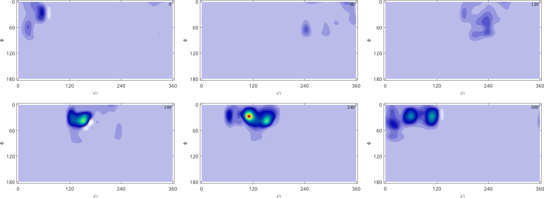
Note that future computations with this SO3FunRBF are also very time consuming, since most methods are faster if the center orientations build a specific grid, which is not the case here.
The interpolation is done by lsqr. Hence the error is dependent from the termination conditions and not in machine precision.
norm(SO3F.eval(ori) - S.values) / norm(S.values)ans =
9.0528e-04Also, interpolation might not guarantee non-negativity of the function
minValue = min(SO3F)minValue =
-7.6067LSQR-Parameters
The lsqr solver and the mlsq solver, which are used to minimize the least squares problem from above has some predefined termination conditions. We can specify the method tolerance with the option 'tol' (default 1e-3) and the maximum number of iterations by the option 'maxit' (default 30/100).
Thus we are able to control the precision of the result and computational time of the least squares methods in the approximation process.
% default Parameters
tic
[f1,iter1] = SO3FunRBF.interpolate(ori, val);
toc
fprintf(['Number of iterations = ',num2str(iter1),'\n', ...
         'Value of energy functional = ',num2str(norm(f1.eval(ori)-val)),'\n\n'])

% new termination conditions
tic
[f2,iter2] = SO3FunRBF.interpolate(ori, val,'tol',1e-15,'maxit',100);
toc
fprintf(['Number of iterations = ',num2str(iter2),'\n', ...
         'Value of energy functional = ',num2str(norm(f2.eval(ori)-val)+5e-7*norm(f2,2)),'\n'])
Elapsed time is 0.346294 seconds.
Number of iterations = 8
Value of energy functional = 0.43171
Elapsed time is 0.447571 seconds.
Number of iterations = 41
Value of energy functional = 0.0015935