Texture Evolution

Plastic deformation changes both the shape and the crystallographic texture of a polycrystal. Under the Taylor model, each crystal accommodates the same imposed strain by slip and rotates as it does so. Repeating that rotation for small strain increments produces a simple simulation of texture evolution.

Import from VPSC showed how to read a deformation history computed outside MTEX. Here the history is computed inside MTEX. The Single Slip Model instead solves the ODF continuity equation for independently slipping crystals.

Define the deformation model

We use the {111}<110> slip systems of a face-centred cubic crystal. Slip Systems explains the plane, direction, and symmetrization represented by this list.

cs = crystalSymmetry('432');
sS = symmetrise(slipSystem.fcc(cs));

Plane strain is a simple model for rolling. The strain extends the first specimen axis, leaves the second unchanged, and shortens the third by the same amount. The parameter \(q\) can distribute the shortening between the second and third axes; here \(q=0\) gives plane strain.

q = 0;
epsTotal = 0.6 * strainTensor(diag([1 -q -(1-q)]));

Rotate one crystal

A spin tensor describes an infinitesimal rotation. For one oriented crystal, calcTaylor returns the Taylor factor M, the slip amounts, and the crystallographic spin W required by the imposed strain increment.

Slip systems live in the crystal frame. The inverse orientation therefore expresses the specimen strain in that frame before the Taylor solve.

oriSingle = orientation.byEuler(0,30*degree,15*degree,cs);
epsStep = 0.01 * strainTensor(diag([1 -q -(1-q)]));

[M,~,W] = calcTaylor(inv(oriSingle) * epsStep,sS);
M
W

M =
    2.3153
 
W = spinTensor (crystal)
  rank: 2 (3 × 3)
 
 *10^-4
      0 -47.11 -68.65
  47.11      0  24.65
  68.65 -24.65      0

Applying the negative crystallographic spin updates the orientation. The angle below measures the resulting orientation change.

oriNew = exp(oriSingle,-W);
rotationAngle = angle(oriSingle,oriNew) ./ degree

rotationAngle =
    0.4975

One percent strain gives a Taylor factor of 2.3153 and rotates this crystal by 0.4975 degrees. Spin depends on orientation, so crystals in a polycrystal follow different paths and this example develops texture.

Compute an orientation-dependent spin field

Solving the Taylor problem separately at every sampled orientation would be slow. When the strain remains in the specimen frame, calcTaylor returns the Taylor factor and spin as orientation-dependent functions. The expensive field can then be evaluated cheaply at an entire list of orientations.

Divide the total strain into 60 increments and compute the corresponding spin field once. The Taylor solution is positively homogeneous in strain, so the same incremental field is used at every step.

numIter = 60;
[~,~,spin] = calcTaylor(epsTotal ./ numIter,sS)

spin = SO3VectorFieldHarmonic (1 → y↓→x)
  bandwidth: 32
  tangent space: rightSpinTensor
  intern symmetries: 432 → y↓→x
  intern tangent space: leftVector

This calculation takes most of the page's run time. Its cost depends on the bandwidth of the harmonic representation rather than on the later number of sampled orientations. Passing 'bandwidth',16 is noticeably faster, at the price of a relative spin-field error of a few percent.

Start from a uniform texture

The 20,000 random orientations approximate a uniform texture, whose texture index \(\lVert f\rVert^2\) is close to 1.

ori = orientation.rand(2e4,cs);
odf0 = calcDensity(ori,'halfwidth',10*degree);
initialTextureIndex = norm(odf0)^2

initialTextureIndex =
    1.0008

Step through the strain history

At every increment, evaluate the spin at the current orientations and move them by that rotation. The spin field returns right-sided spin tensors in crystal coordinates, which fixes the order and sign in exp. We retain the orientations after 20, 40, and 60 steps so their texture indices can be compared later.

oriAtStep = cell(1,3);
pC = progressCounter(numIter);
for k = 1:numIter
  W = spin.eval(ori);
  ori = exp(ori,-W);

  if mod(k,20) == 0
    oriAtStep{k/20} = ori;
  end
  pC.show(k);
end

Read the resulting rolling texture

The result lives in the rolling specimen frame. This frame names the axes rolling direction (RD), transverse direction (TD), and normal direction (ND). Its plotting convention places RD north, TD west, and ND out of the page.

previousFrame = specimenFrame.default;
specimenFrame.rolling.makeDefault

plotPDF(ori,Miller({0,0,1},{1,1,1},cs),'contourf')
mtexColorbar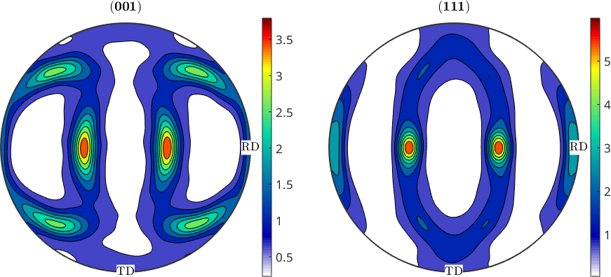

The initially diffuse poles have gathered into several symmetry-related maxima. Their concentrated contours are the pole-figure signature of the fcc rolling components generated by the Taylor rotations.

Measure texture strength

The texture index is 1 for a uniform ODF and grows as orientation density becomes more concentrated. Compute it at 0, 20, 40, and 60 percent strain with the same density-estimation halfwidth, so the values are comparable.

textureIndex = initialTextureIndex;
for k = 1:3
  odfAtStep = calcDensity(oriAtStep{k},'halfwidth',10*degree);
  textureIndex(k+1) = norm(odfAtStep)^2;
end

strainPercent = [0 20 40 60];
table(strainPercent.',textureIndex.',...
  'VariableNames',{'StrainPercent','TextureIndex'})

ans =
  4×2 table
    StrainPercent    TextureIndex
    _____________    ____________
          0             1.0008   
         20              1.144   
         40             1.4874   
         60             1.9036

The index rises from 1.0010 initially to 1.1499, 1.4984, and 1.9160. This steady increase quantifies the sharpening seen in the pole figures, although the ODF is not yet extremely concentrated at 60 percent strain.

odf = odfAtStep;
plotSection(odf,'phi2',[0 45 65]*degree,'contourf')
mtexColorbar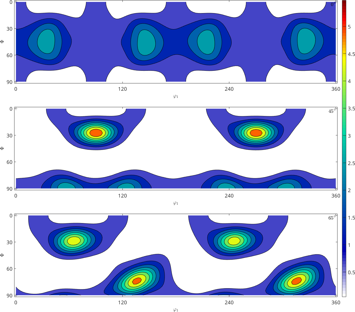

The same orientation-density maxima now appear in three phi2 sections. Their compact patches, separated by broad low-density regions, show where the rolling texture is concentrated in the three-dimensional ODF.

% Restore the incoming session frame after the published figures are made.
specimenFrame.default(previousFrame);

Numerical and physical limits

References

Next

Taylor Model for Hexagonal Materials applies the same Taylor rotation to magnesium in a single large step. It adds slip families with unequal critical resolved shear stresses and compares two temperatures.

References

- G. I. Taylor, Plastic Strain in Metals, Journal of the Institute of Metals 62 (1938), 307--324. This paper introduces the equal-strain polycrystal model used for every orientation update.
- H.-J. Bunge, Some applications of the Taylor theory of polycrystal plasticity, Kristall und Technik 5 (1970), 145--175. This paper develops the orientation-dependent Taylor factor and crystallographic spin used here.