Import from VPSC

Import from VPSC edit page

VPSC is a crystal plasticity code originally written by Ricardo Lebensohn and Carlos Tome from Los Alamos National Laboratory - USA.

Original code can be requested to lebenso@lanl.gov

https://public.lanl.gov/lebenso/

Import the orientations generated by VPSC

Running a simulation in VPSC usually results in an output file TEX_PH1.OUT which contains multiple sets of orientations for different strain levels. As these files does not contain any information on the crystal symmetry we need to specify it first

cs = crystalSymmetry('222', [4.762 10.225 5.994],'mineral', 'olivine');

In the next step the orientations are imported and converted into a list of ODFs using the command ODF.load.

% put in here the path to the VPSC output files
path2file = [mtexDataPath filesep 'VPSC'];

odf = SO3Fun.load([path2file filesep 'TEX_PH1.OUT'],'halfwidth',10*degree,'CS',cs)

odf =
  1×9 cell array
  Columns 1 through 3
    {1×1 SO3FunHarmonic}    {1×1 SO3FunHarmonic}    {1×1 SO3FunHarmonic}
  Columns 4 through 6
    {1×1 SO3FunHarmonic}    {1×1 SO3FunHarmonic}    {1×1 SO3FunHarmonic}
  Columns 7 through 9
    {1×1 SO3FunHarmonic}    {1×1 SO3FunHarmonic}    {1×1 SO3FunHarmonic}

The individual ODFs can be accessed by odf{id}

% lets plot the second ODF
plotSection(odf{2},'sigma','figSize','normal')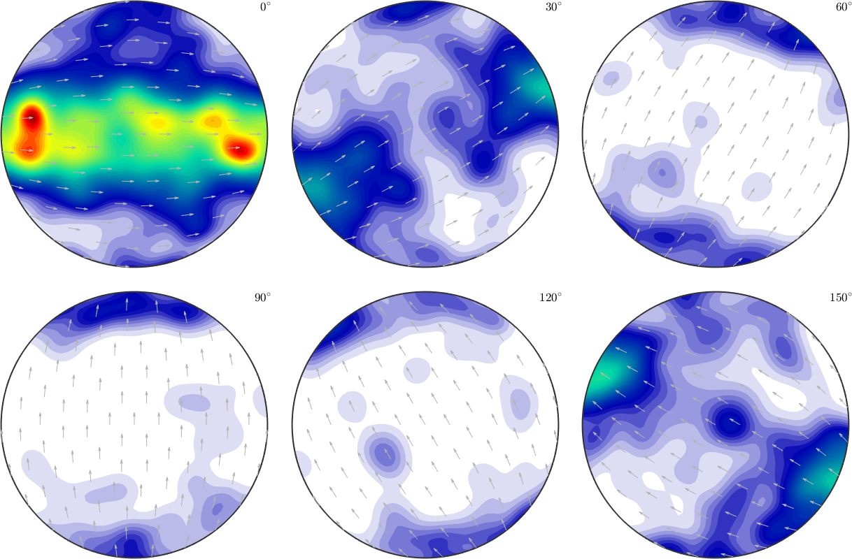

The information about the strain are stored as additional properties within each ODF variable

odf{1}.opt

ans = 
  struct with fields:

                   strain: 0.2500
          strainEllipsoid: [1.1230 1.1270 0.7500]
    strainEllipsoidAngles: [-180 90 -180]
             orientations: [1000×1 orientation]
                     data: [1000×3 double]

Compare pole figures during deformation

Next we examine the evaluation of the ODF during the deformation by plotting strain depended pole figures.

% define some crystal directions
h = Miller({1,0,0},{0,1,0},{0,0,1},cs,'uvw');

% generate some figure
fig = newMtexFigure('layout',[4,3],'figSize','huge');
subSet = 1:4;

% plot pole figures for different strain steps
for n = subSet
  nextAxis
  plotPDF(odf{n},h,'lower','contourf','doNotDraw');
  ylabel(fig.children(end-2),['\epsilon = ',xnum2str(odf{n}.opt.strain)]);
end
setColorRange('equal')
mtexColorbar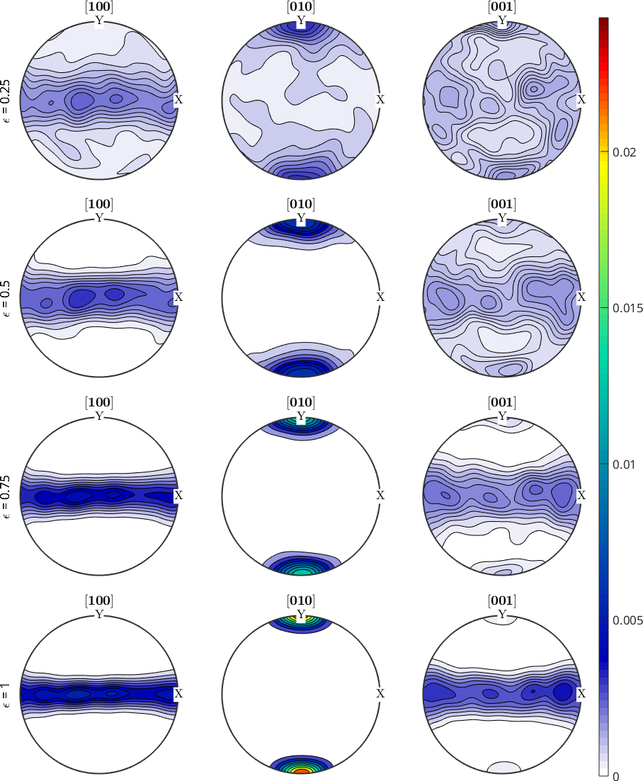

Visualize slip system activity

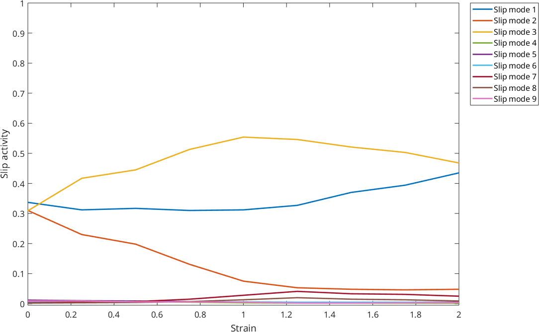
Alongside with the orientation data VPSC also outputs a file ACT_PH1.OUT which contains the activity of the different slip systems during the deformation. Lets read this file as a table

ACT = readtable([path2file filesep 'ACT_PH1.OUT'],'FileType','text')

ACT =
  9×11 table
    STRAIN    AVACS    MODE1    MODE2    MODE3    MODE4    MODE5    MODE6    MODE7    MODE8    MODE9
    ______    _____    _____    _____    _____    _____    _____    _____    _____    _____    _____
        0     2.835    0.337     0.31    0.309    0.011    0.012    0.007    0.003    0.002    0.009
     0.25     2.766    0.312     0.23    0.417    0.009     0.01    0.007    0.005    0.003    0.009
      0.5     2.835    0.317    0.198    0.445    0.007    0.009    0.007    0.007    0.004    0.006
     0.75     2.825     0.31    0.131    0.513    0.005    0.007    0.006    0.015    0.007    0.006
        1     2.759    0.312    0.075    0.554    0.003    0.005    0.006    0.028    0.013    0.005
     1.25     2.746    0.327    0.053    0.546    0.002    0.004    0.005    0.041     0.02    0.002
      1.5     2.736     0.37    0.048    0.521    0.002    0.005    0.005    0.033    0.015    0.002
     1.75     2.739    0.394    0.046    0.503    0.002    0.005    0.005    0.031    0.013    0.003
        2     2.828    0.435    0.048    0.468    0.002    0.005    0.004    0.025    0.009    0.004

and plot the slip activity with respect to the strain for the different modes

% loop though the columns MODE1 ... MOD11
close all
for n = 3: size(ACT,2)

  % perform the plotting
  plot(ACT.STRAIN, table2array(ACT(:,n)),'linewidth',2,...
    'DisplayName',['Slip mode ',num2str(n-2)])
  hold on;
end
hold off

% some styling
xlabel('Strain');
ylabel('Slip activity');
legend('show','location','NorthEastOutside');

set(gca,'Ylim',[-0.005 1])
set(gcf,'MenuBar','none','units','normalized','position',[0.25 0.25 0.5 0.5]);

%for only one mode plot, e.g.,mode 3: cs = csapi(STRAIN,MODE{3});fnplt(cs,3,'color','b');hold off;