Pole figures are two dimensional representations of orientations. To illustrate this we define a random orientation with trigonal crystal symmetry
cs = crystalSymmetry('321')
ori = orientation.rand(cs)
cs = crystalSymmetry
symmetry : 321
elements : 6
a, b, c : 1, 1, 1
reference frame: X||a*, Y||b, Z||c*
ori = orientation (321 → y↑→x)
Bunge Euler angles in degree
phi1 Phi phi2
156.958 161.468 197.878Starting point is a fixed crystal direction h, e.g.,
% the fixed crystal directions (100)
h = Miller({1,0,0},cs);
Next the specimen directions corresponding to all crystal directions symmetrically equivalent to h are computed
r = ori * h.symmetriser = vector3d (y↑→x)
size: 1 x 6
x y z
0.88 -0.739 -0.113
1.08 0.34 0.246
-1.08 -0.34 -0.246
-0.88 0.739 0.113
0.196 1.08 0.359
-0.196 -1.08 -0.359and plotted in a spherical projection
plot(r)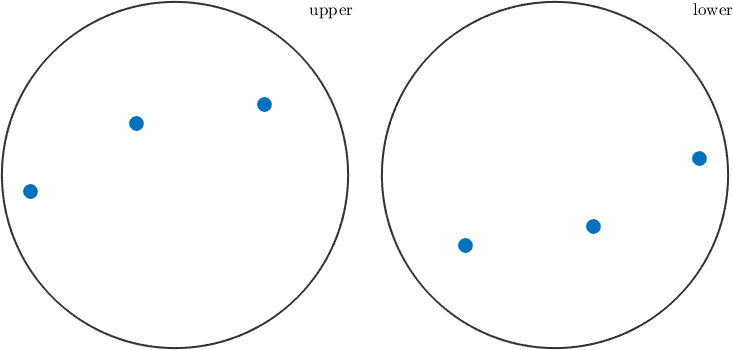
Since the trigonal symmetry group has six symmetry elements the orientation appears at six positions.
A shortcut for the above computations is the command
% a pole figure plot
plotPDF(ori,Miller({1,0,-1,0},{0,0,0,1},{1,1,-2,1},ori.CS))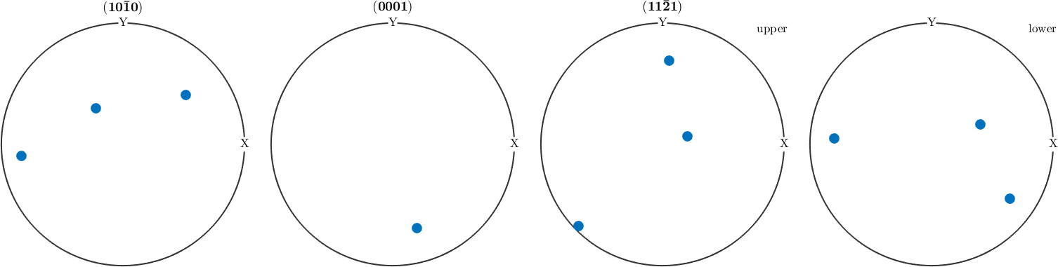
We observe, that for some crystal directions only the upper hemisphere is plotted while for other upper and lower hemisphere are plotted. The reason is that if h and -h are symmetrically equivalent the upper and lower hemisphere of the pole figure are symmetric as well.
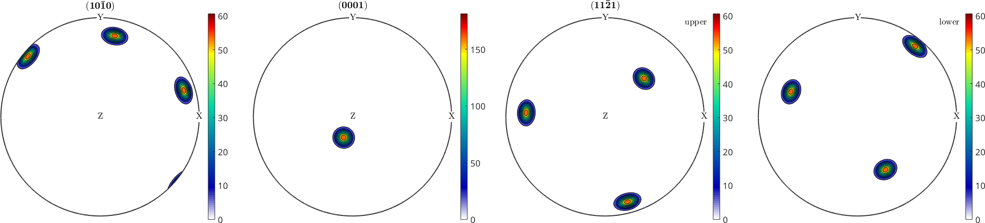
Contour plots
plotPDF(ori,Miller({1,0,-1,0},{0,0,0,1},{1,1,-2,1},ori.CS),'contourf')
mtexColorbar