Importing EBSD Data

An EBSD map represents a list of measurements, whatever layout the file uses on disk. Each measurement has a position, a phase and an orientation. Importing turns that list into an EBSD variable and supplies the crystallography and reference frames needed to interpret it.

Before starting, identify the specimen directions and check the phase names, lattice parameters and crystal-axis alignments reported by the acquisition software. Orientations explains how an orientation relates the crystal and specimen frames.

EBSD.load chooses the interface from the file extension. The first import needs only a filename.

plottingConvention.default('y↓→x');

fileName = [mtexEBSDPath filesep 'EMSphinx.h5'];
ebsd = EBSD.load(fileName)

════════════════════════════════════════════════════════════════════════════════
HDF5 CONFIGURATION LOADED
├── Manufacturer : EMSphInx
├── Data sets    : 4
│   ▸ [1] Scan 1/EBSD
│     [2] Scan 2/EBSD
│     [3] Scan 3/EBSD
│     [4] Scan 4/EBSD
└── Pick one by EBSD.load(fname,'dataSet',4) or 'dataSet','Scan 4/EBSD'
════════════════════════════════════════════════════════════════════════════════
 
ebsd = EBSDsquare (y↓→x, row↓→col)
 
 Phase  Orientations           Mineral         Color  Symmetry  Crystal reference frame
     0  2148 (0.44%)    Fe(alpha-iron)  LightSkyBlue      m-3m                         
     1  478052 (99%)    Fe(gamma-iron)  DarkSeaGreen      m-3m                         
     2     4940 (1%)  Co(alpha-cobalt)     Goldenrod     6/mmm        X||a, Y||b*, Z||c
 
 Properties: IQ, Metric, oldId
 Scan unit : um
 X × Y × Z : [0 → 382] × [0 → 203] × [0 → 0]
 Normal vector: (0,0,1)
 Square grid  :508 × 955
 dataSet: /Scan 1/EBSD
 dataSets: Scan 1/EBSD Scan 2/EBSD Scan 3/EBSD Scan 4/EBSD

Read this display once. It is the inventory for everything that follows. The file contains four scans, and the triangle in the data-set list marks the first as the one imported. Three indexed phases arrived with lattice parameters, and the cobalt phase states its crystal-axis alignment. Two phases are cubic, and 99% of the measurements are gamma iron. The square grid has 508 × 955 cells and covers about 382 × 203 microns.

The display also lists IQ, Metric and oldId as properties. A property has one value per measurement and is subset together with the map. By contrast, the selected HDF5 path and the file header are scan-level options under ebsd.opt; they are not resized by a selection.

A phase map is the quickest check that the scan footprint and phase inventory are plausible.

plot(ebsd)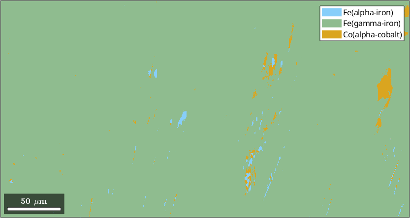

Almost the entire map has the gamma-iron phase colour, as the 99% figure predicts. The sparse alpha-iron and cobalt measurements remain visible against it, so a wrong phase identifier would not be hidden by the total.

This variable is the starting point for grain reconstruction, ODF estimation and misorientation analysis.

What Import Cannot Guess

A reference frame is the coordinate system in which data are expressed. Two reference frames can be involved in an EBSD measurement: the frame of the map coordinates and the frame used for the Euler angles. Vendors align them differently, and a file does not always record their relationship.

The failure mode is quiet. A map imported with the wrong relationship still plots, still reconstructs into grains and still yields pole figures. Those results are simply rotated or mirrored with respect to the specimen, and no number in the data set reveals the mistake.

A plotting convention only states how a reference frame is laid out on screen. Changing it can turn the displayed map, but it cannot repair an incorrect relationship between the two frames. Supply that relationship during import, then follow Reference Frame Alignment to validate it against a known specimen direction or microstructural feature.

The Import Wizard

The wizard is the interactive route through those choices. Start it with import_wizard. It works with EBSD, pole figure and ODF data.

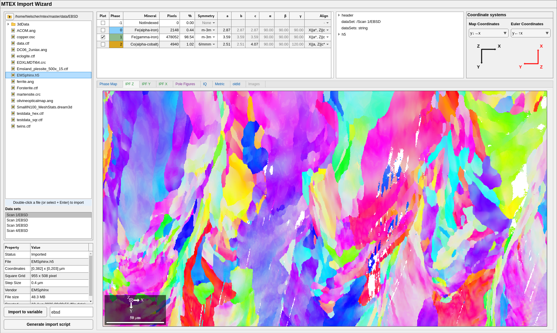
Notice how the selected data set at lower left, the phase table across the top, and the map and Euler coordinate selectors at upper right are shown together. Changing an alignment redraws the map, so you can compare the result with the specimen rather than guess a vendor convention.

The wizard can create the variable directly, but its more useful output is an import script. The script records every choice, runs without the wizard and provides a reproducible start for the rest of the analysis.

The Import Script

The essential part of a generated script is shown below. It records the phases, the screen alignment, the source file, the frame correction and a first plot.

% crystal symmetry
csList = [
  notIndexed(), ...
  crystalSymmetry('m-3m', [2.8665 2.8665 2.8665], ...
    'mineral', 'Fe(alpha-iron)', 'color', 'LightSkyBlue'), ...
  crystalSymmetry('m-3m', [3.591 3.591 3.591], ...
    'mineral', 'Fe(gamma-iron)', 'color', 'DarkSeaGreen'), ...
  crystalSymmetry('6/mmm', [2.5071 2.5071 4.0686], ...
    'mineral', 'Co(alpha-cobalt)', 'color', 'Goldenrod', ...
    'X||a', 'Y||b*', 'Z||c')
];

% how the map is aligned on screen
pC = plottingConvention('y↓→x');

% path to files
pname = mtexEBSDPath;

% which files to be imported
fname = [pname filesep 'EMSphinx.h5'];

% rotates the Euler angle reference frame onto the map reference frame
EulerCorrection = rotation.map(xvector,xvector,zvector,-zvector);

% create an EBSD variable containing the data
ebsd = EBSD.load(fname,csList,'dataSet',1, ...
  'EulerCorrection',EulerCorrection,pC,'silent');

% everything derived later that states no frame of its own follows this
plottingConvention.default('y↓→x');

The crystal-symmetry calls state both a point group and a crystal frame. For cobalt, the X parallel a, Y parallel b-star and Z parallel c choices align the Cartesian crystal frame with the lattice basis; they are not part of the 6/mmm point group.

EulerCorrection is a frame change from the Euler-angle frame to the map frame. Here it maps Euler \(x\) onto map \(x\) and Euler \(z\) onto minus map \(z\). This is the correction for a map with \(y\) pointing down when the Euler angles were measured with \(y\) pointing up.

The convention pC is also passed into the import. Data in a named specimen frame carries that frame's plotting convention and would not otherwise follow a later session default.

The wizard ends with an orientation plot. Unlike the phase map above, this plot checks that orientations and positions have arrived together as a spatially coherent map.

plot(ebsd('Fe(gamma-iron)'),ebsd('Fe(gamma-iron)').orientations, ...
  'ipfDirection',zvector)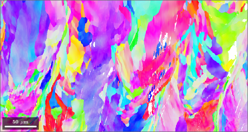

Coherent elongated domains and smooth colour changes inside them show that the orientations have not been scrambled across the scan. An equally coherent map can still be rotated or mirrored, so this picture alone does not validate the reference frame. Use the known-direction tests on Reference Frame Alignment for that.

Supported Data Formats

The HDF5 interface reads Bruker, EDAX, Oxford, ThermoFisher, EMsoft and EMSphInx layouts. Prefer a documented, non-proprietary format when the acquisition software offers one. A published specification preserves the units, hierarchy and coordinate definitions needed to read the data later. Add a new HDF5 layout through the JSON configuration described in HDF5 Interface rather than writing another HDF5 reader.

The generic loader is the fallback for a text file that no vendor interface recognises. If it contains Euler angles, a phase and spatial coordinates as columns,

alpha_1 beta_1 gamma_1 phase_1 x_1 y_1
alpha_2 beta_2 gamma_2 phase_2 x_2 y_2
alpha_3 beta_3 gamma_3 phase_3 x_3 y_3
.       .      .       .       .   .
alpha_M beta_M gamma_M phase_M x_M y_M

then the wizard lets you assign each column. Orientations without spatial coordinates do not form a map; import them as described in Importing Orientations.

HDF5 Files With Several Data Sets

An HDF5 project file can hold more than one map. EDAX paths commonly contain Area N/OIM Map N, Oxford uses numbered slices, and EMSphInx uses Scan N. The opening import prints every available data set and marks the selected one. When no selection is supplied, the first entry is imported.

Select another by its one-based number or by an unambiguous part of its name.

ebsd = EBSD.load(fname,'dataSet',2)
ebsd = EBSD.load(fname,'dataSet','OIM Map 7')

The full imported HDF5 path is the scan-level option ebsd.opt.dataSet. The short names of all choices are stored in ebsd.opt.dataSets.

To inspect a large file without reading its per-pixel arrays, use

ebsd = EBSD.load(fname,'headerOnly')

This returns an empty measurement list but still fills the phase list, phase map and ebsd.opt.header. A header is the scan-level information from the file preamble, such as acquisition settings and vendor records. Its field names retain the vendor's native layout; MTEX does not impose a common header schema. The available HDF5 data sets are listed as well.

The import wizard uses this lightweight preview below its file browser. Selecting a row then imports that data set.

Raw and Post-Processed Data

An Oxford h5oina file may store the same map twice: as recorded by the detector under EBSD and after vendor processing under Data Processing. They are two data sets of one file. MTEX lists them together and puts the processed version first.

ebsd = EBSD.load(fname)                        % post-processed
ebsd = EBSD.load(fname,'dataSet','EBSD')       % as recorded

The recorded version usually retains more per-pixel properties, such as band contrast, band slope, pattern quality and pattern-centre values. The processed version may retain fewer properties but includes the vendor's bad-pixel cleanup. Both refer to the same specimen frame, so their orientations can be compared directly.

A file that was never processed contains the recorded version alone and lists one data set per map.

Writing Your Own Interface

A format not covered above needs a loader function. The established name is loadEBSD_xxx.m, and the loaders in mtex/interfaces are examples. Return an EBSD variable and call the new function directly while developing it.

Current EBSD.load dispatch is explicit: placing a function in that folder does not by itself register a new extension. Full integration also requires adding the extension to EBSDExtensions and a dispatch case to EBSD.load. The import wizard uses the same extension list to decide which files it offers as EBSD data.

References

Next

Continue with Reference Frame Alignment before trusting any specimen-relative result. Then use Plotting to inspect map quantities and Selecting EBSD Data to restrict the measurement list. Exporting EBSD Data covers writing the checked map back to disk.

References

- A. J. Schwartz, M. Kumar, B. L. Adams and D. P. Field, editors, Electron Backscatter Diffraction in Materials Science, second edition, Springer, 2009, develops EBSD measurement, calibration and orientation mapping.
- T. B. Britton et al., Tutorial: Crystal orientations and EBSD -- Or which way is up?, Materials Characterization 117, 113--126, 2016, gives a practical calibration chain between detector, scan, specimen and crystal frames.
- ISO 24173:2024, Microbeam analysis -- Guidelines for orientation measurement using electron backscatter diffraction, specifies current guidance for reproducible orientation measurements, including specimen alignment and calibration.
- M. A. Jackson et al., h5ebsd: an archival data format for electron back-scatter diffraction data sets, Integrating Materials and Manufacturing Innovation 3, 44--55, 2014, defines a vendor-neutral HDF5 archival layout.
- The Oxford Instruments NanoAnalysis HDF5 File Specification documents the public
h5oinahierarchy, units and coordinate systems used by that format.