Spherical Kernel Functions

A spherical kernel \(\psi\) is a spherical function that depends only on the angle towards the north pole \(e_3\),

psi = S2DeLaValleePoussinKernel('halfwidth',10*degree)

surf(psi,'resolution',2*degree,'EdgeColor','none')
hold on
arrow3d(2.4*zvector,'labeled','arrowwidth',0.01)
hold off
axis off

psi = S2DeLaValleePoussinKernel
  bandwidth: 25
  halfwidth: 10°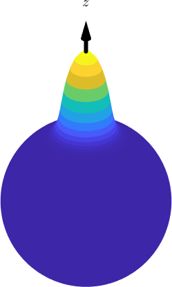

The dependency of the angle becomes more when plot along meridian

close all
plot(psi,'linewidth',2,'symmetric')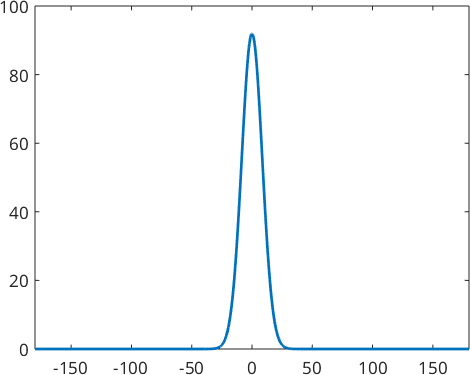

Examples of spherical kernel functions are

Legendre coefficients

Every spherical kernel function \(\psi\) can be associated with a function \(\Psi \colon [-1,1] \to \mathbb R\) defined on the interval \([-1,1]\) by \(\psi(v) = \Psi(v \cdot e_3)\). It turn out to be useful to \(\Psi\) approximate \(\Psi\) by a expansion into Legendre polynomials \(P_n\) of degree \(n\), i.e.,

\[ \psi(t) = \sum\limits_{n=0}^{\infty} \hat\psi_n \, \mathcal P_{n}(t) \]

These Legendre coefficients are stored as the field psi.A and can be easily visualized using the command plotSpectra.

plotSpektra(psi,'linewidth',2)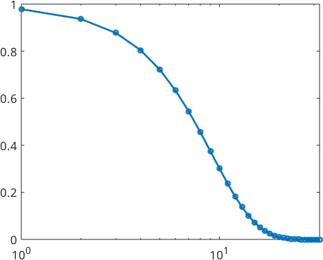

Applications

Spherical kernel functions have different applications in MTEX. Those include

The de la Vallee Poussin Kernel

The spherical de la Vallee Poussin kernel is defined by

\[ K(t) = (1+\kappa)\,(\frac{1+t}{2})^{\kappa}\]

for \(t\in[0,1]\). The de la Vallee Poussin kernel additionally has the unique property that for a given halfwidth it can be described exactly by a finite number of Fourier coefficients. This kernel is recommended for Texture analysis as it is always positive and there is no truncation error in Fourier space.

Hence we can define the de la Vallee Poussin kernel \(\psi_{\kappa}\) depending on a parameter \(\kappa \in \mathbb N \setminus \{0\}\) by its finite Legendre polynomial expansion

\[ \psi_{\kappa}(t) = \sum\limits_{n=0}^{L} a_n(\kappa) \mathcal P_{n}(t).\]

We obtain the Legendre coefficients \(a_n(\kappa)\) by \(a_0=1\), \(a_1=\frac{\kappa}{2+\kappa}\) and the three term recurrence relation

\[ (\kappa+l+2) a_{l+1} = -(2l+1)\,a_l + (\kappa-l+1)\,a_{l-1}.\]

Lets construct two of them.

psi1 = S2DeLaValleePoussinKernel('halfwidth',15*degree)
psi2 = S2DeLaValleePoussinKernel('halfwidth',20*degree)

plot(psi1,'linewidth',2,'symmetric')
hold on
plot(psi2,'linewidth',2,'symmetric')
hold off
legend('halfwidth = 15°','halfwidth = 20°')

psi1 = S2DeLaValleePoussinKernel
  bandwidth: 17
  halfwidth: 15°
 
 
psi2 = S2DeLaValleePoussinKernel
  bandwidth: 13
  halfwidth: 20°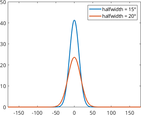

Here the parameter \(\kappa\) is \(40.34\) for function \(\psi_1\) and \(22.64\) in function \(\psi_2\).

We also take a look at the Legendre coefficients

plotSpektra(psi1,'linewidth',2)
hold on
plotSpektra(psi2,'linewidth',2)
hold off
legend('halfwidth = 15°','halfwidth = 20°')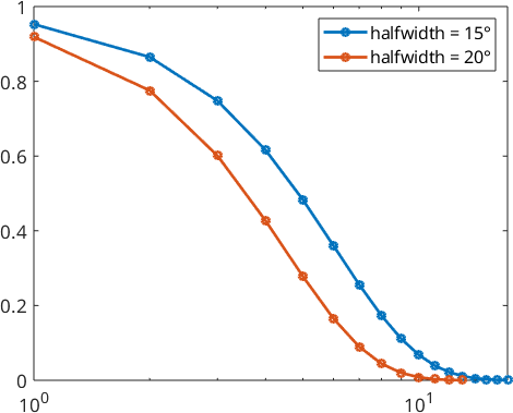

The Dirichlet Kernel

The spherical Dirichlet or Christoffel-Darboux kernel is recommended for calculating physical properties as the Legendre coefficients always have a value of one up to the specified bandwidth:

\[ \psi_N(t) = \sum\limits_{n=0}^N (2n+1) \, \mathcal P_{n}(t).\]

Lets construct two of them.

psi1 = S2DirichletKernel(10)
psi2 = S2DirichletKernel(5)

plot(psi1,'linewidth',2,'symmetric')
hold on
plot(psi2,'linewidth',2,'symmetric')
hold off
legend('bandwidth = 5','bandwidth = 10')

psi1 = S2DirichletKernel
  bandwidth: 10
  halfwidth: 180°
 
 
psi2 = S2DirichletKernel
  bandwidth: 5
  halfwidth: 180°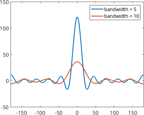

By looking at the Legendre coefficients we see, that they are exactly 1.

plotSpektra(psi1,'linewidth',2)
hold on
plotSpektra(psi2,'linewidth',2)
hold off
legend('bandwidth = 5','bandwidth = 10')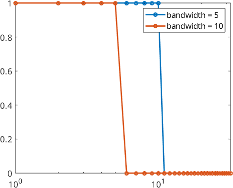

The Bump kernel

The spherical bump kernel is a radial symmetric kernel function depending on the halfwidth \(r\in (0,pi)\). The function value is 0, if the angle is greater then the halfwidth \(r\). Otherwise it is 1.

The main problem of the bump kernel is that we need lots of Legendre coefficients to describe it. That possibly can result in high runtimes.

psi1 = S2BumpKernel(30*degree)
psi2 = S2BumpKernel(50*degree)

plot(psi1,'linewidth',2,'symmetric')
hold on
plot(psi2,'linewidth',2,'symmetric')
hold off
legend('halfwidth = 30°','halwidth = 40°')

psi1 = S2BumpKernel
  bandwidth: 2000
  halfwidth: 30°
 
 
psi2 = S2BumpKernel
  bandwidth: 2000
  halfwidth: 50°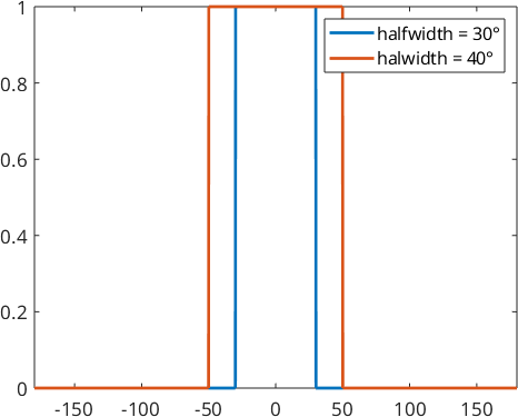

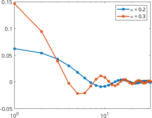
We also take a look at the Fourier coefficients

plotSpektra(psi1,'linewidth',2)
hold on
plotSpektra(psi2,'linewidth',2)
hold off
legend('\kappa = 0.2','\kappa = 0.3')