ODF Tutorial

Theory

The orientation distribution function (ODF) is a function in orientation space that associates each orientation \(g\) with the volume fraction of crystals in a polycrystalline specimen that are in this specific orientation, i.e.,

\[\mathrm{odf}(g) = \frac{1}{V} \frac{\mathrm{d}V(g)}{\mathrm{d}g}.\]

In MTEX a perfectly random texture will have an ODF equal to one for all orientations. In other words the values of ODFs in MTEX can be interpreted as multiples of the random distribution (mrd).

Computing an ODF from Individual Orientations

Individual orientation data may be obtained experimentally by EBSD (orientation mapping in a SEM), ACOM (orientation mapping in a TEM) or 3d X-ray imaging; or from simulations, like VPSC. In the following we consider an EBSD map of a Titanium alloy. Note that this data set is measured on a hexagonal grid rather than the more common square grid.

% import the titanium data
mtexdata titanium

% plot an orientation map
plot(ebsd, ebsd.orientations)

ebsd = EBSDhex (y↓→x)
 
 Phase  Orientations           Mineral         Color  Symmetry  Crystal reference frame
     0    8100 (99%)  Titanium (Alpha)  LightSkyBlue       622        X||a, Y||b*, Z||c
 
 Properties: ci, grainid, iq, sem_signal, oldId
 Scan unit : um
 X x Y x Z : [0 → 996] x [0 → 998] x [0 → 0]
 Normal vector: (0,0,1)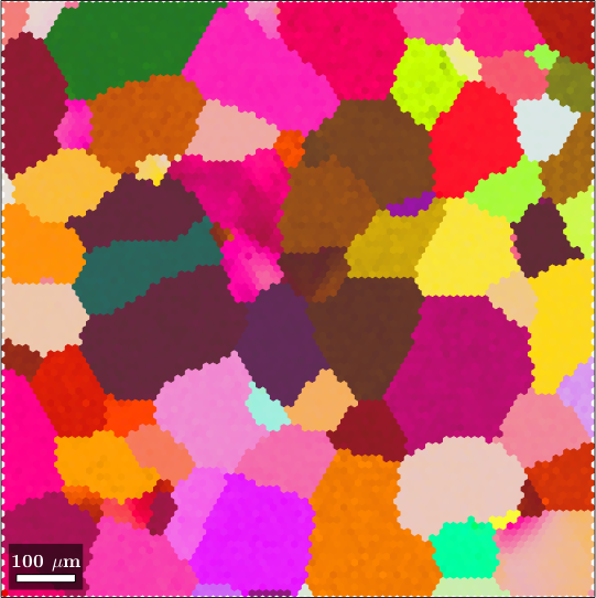
 Hex grid     :97 x 84

Computing an ODF from individual orientations is done by kernel density estimation using the command calcDensity.

% extract the orientations
ori = ebsd.orientations;

% compute the ODF
odf = calcDensity(ori)

odf = SO3FunHarmonic (Titanium (Alpha) → y↓→x)
  bandwidth: 25
  weight: 1

There are many different ways to visualize an ODF: Euler or sigma sections, three dimensional plots, pole figures and inverse pole figures. The most common but not recommended way are sections with respect to the third Euler angle \(\varphi_2\)

plot(odf)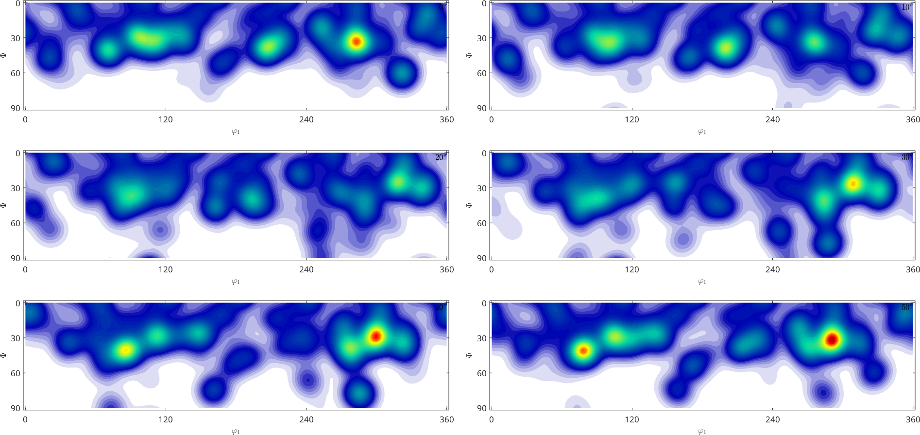

Computing an ODF from Pole Figure Data

Pole figure data arises when textured materials are measured via x-ray, neutron or synchrotron radiation. Generally, for \(3\) to \(10\) diffraction planes specified by Miller indices \((hk\ell)\) diffraction intensities are measured at a spherical grid of specimen directions. In the example below each dot corresponds to one diffraction intensity at the plane indicated at the top of the spherical plots measured from the direction corresponding to the pixel position.

% import pole figure data
plottingConvention.default('y↑→x');
mtexdata ptx

% plot the data
plot(pf)

% show the colour bar - note that the maximum intensity is different for
% each pole figure
mtexColorbar

pf = PoleFigure (y↑→x)
  crystal symmetry : mmm
 
  h = (104), r = 72 x 17 points
  h = (110), r = 72 x 17 points
  h = (202), r = 72 x 17 points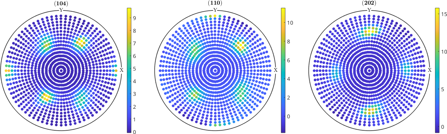

The reconstuction of an ODF from pole figure data requires the solution of an ill posed inverse problem. This means the reconstruction problem has in general not a unique solution, but there are several ODFs that correspond to the same set of pole figure data. MTEX applies some heuristics to identify among all solutions the physically most reasonable.

% compute an ODF with default settings
odf = calcODF(pf)

odf = SO3FunRBF (mmm → y↑→x)
 
  multimodal components
  kernel: de la Vallee Poussin, halfwidth 5°
  center: 29772 orientations, resolution: 5°
  weight: 1

Once an ODF is reconstructed we can check how well its pole figures fit the measured pole figures

% plot the recalculated pole figures
plotPDF(odf,pf.h)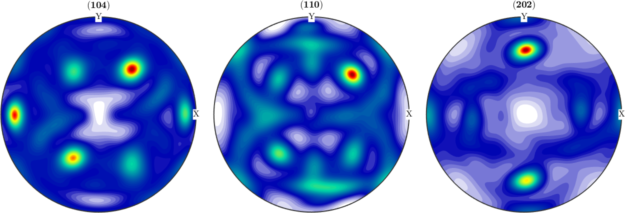

ODF Modeling

Aside from experimental data MTEX also allows the definition of model ODFs of different types. These include unimodal ODFs, fibre ODFs, Bingham Distributed ODFs and any combination of such ODFs.

% define a gamma fibre ODF
odf = fibreODF(fibre.gamma(odf.CS))

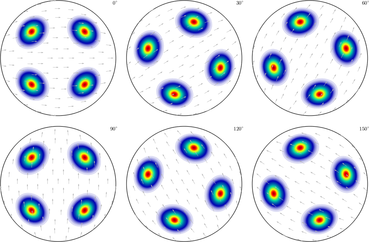
% plot it in sigma sections
plot(odf,'sigma')

odf = SO3FunCBF (mmm → y↑→x)
 
  kernel: de la Vallee Poussin, halfwidth 10°
  fibre : (111) || 0,0,1
  weight: 1