The Bingham distribution on the sphere is an antipodal symmetric distribution (Bingham, 1974) with a probability density function given by
\[p_{b}(\hat{x}\vert AKA^T) = \frac{1}{F(\kappa_{1},\kappa_{2},\kappa_{3})}\exp (\hat{x}^T AZA^T \hat{x})\]
where \(A\) is an orthogonal covariance matrix, and \(Z\) a concentration matrix with \(\mathrm{diag}(\kappa_{1},\kappa_{2},\kappa_{3})\) with \(\kappa_{1} < \kappa_{2} < \kappa_{3}\).
In MTEX \(Z\) is given by Z = [k1,k2,k3] with k3 = 0 and \(A\) is given by three orthogonal vectors.
% A simple example:
Z = [-10 -4 0];
a = rotation.rand(1).*vector3d([xvector yvector zvector]);
bs2 = BinghamS2(Z,a);
plot(bs2)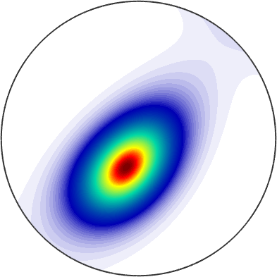
Meaning of \(Z\)
\(k1 = k2\) defines a rotational symmetric point maximum and \(k2 = 0\) defines a girdle distribution.
close
kappa = [0 4 8 12 24];
mtexFig = newMtexFigure('layout',[length(kappa) length(kappa)]);
for k2 = kappa
  for k1 = kappa
    if k1 >= k2
      bs=BinghamS2([-k1 -k2 0]);
      plot(bs,'colorRange',[0,25],'TR',[{'\(\kappa_1 :\)'} ; num2str(k1)],'BR',[{'\(\kappa_2 :\)'} ; num2str(k2)])
%       mtexTitle(['\(\kappa_1 :\)' num2str(k1)  '  ' '\(\kappa_2 :\)' num2str(k2)],'FontSize',14)
      nextAxis
    else
      nextAxis
    end
  end
end
setColorRange('equal')
mtexFig.drawNow;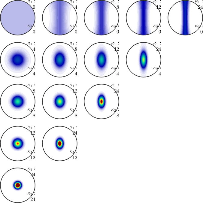
Drawing a random sample of the Bingham distribution
close
v = bs2.discreteSample(500)
plot(bs2)
hold on
plot(v,'MarkerFaceColor','k')
hold off
v = vector3d (y↑→x)
size: 500 x 1
antipodal: true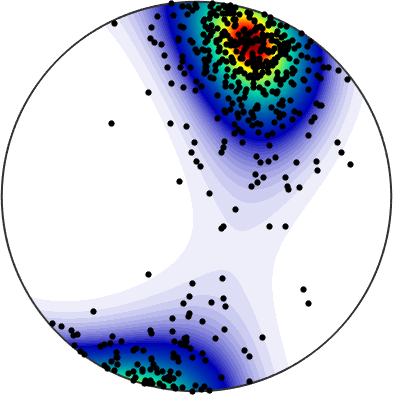
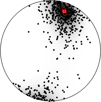
Estimating a spherical Bingham distribution from discrete data
Given arbitrarily scattered data v on the sphere we can estimate the best fitting Bingham distribution by
% estimate a Bingham distribution
bs = BinghamS2.fit(v,'confElli',0.9)
bs = BinghamS2 (y↑→x)Lets plot the fitted distribution with the data
plot(bs)
hold on
plot(v,'MarkerFaceColor','Black')
hold off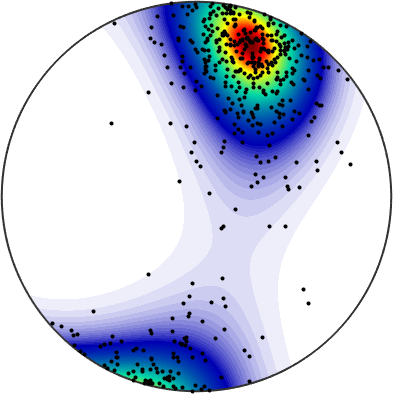
Under the assumption of sufficiently many and sufficently concetrated data we may also estimate a confidence ellipse for the mean direction (default p = 0.95). The center of the ellipse is given by the largest principle vector stored in bs.a(3)
annotate(bs.a(3),'MarkerFaceColor','red','MarkerSize',10)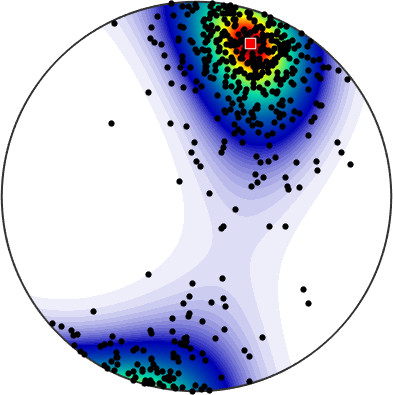
The orientation of the ellipse is specified by all the principle vectors bs.a and the a and b axes are computed by the command cEllipse
mtexColorMap white2black

% annotate the ellipse
ellipse(rotation('matrix',bs.a.xyz'),bs.cEllipse(1),bs.cEllipse(2), ...
    'linewidth',2,'lineColor','r','linestyle','-.')