Martensite Parent Grain Reconstruction

Martensite Parent Grain Reconstruction edit page

This script demonstrates the tools MTEX offers to reconstruct a parent austenite phase from a measured martensite phase. The methods are described in more detail in the publications

The variant graph approach to improved parent grain reconstruction, arXiv, 2022,
Parent grain reconstruction from partially or fully transformed microstructures in MTEX, J. Appl. Cryst. 55, 2022.

We shall use the following sample data set.

% load the data
mtexdata martensite
plotx2east

% grain reconstruction
[grains,ebsd.grainId] = calcGrains(ebsd('indexed'), 'angle', 3*degree, 'minPixel',2);
grains = smooth(grains,5);

% plot the data and the grain boundaries
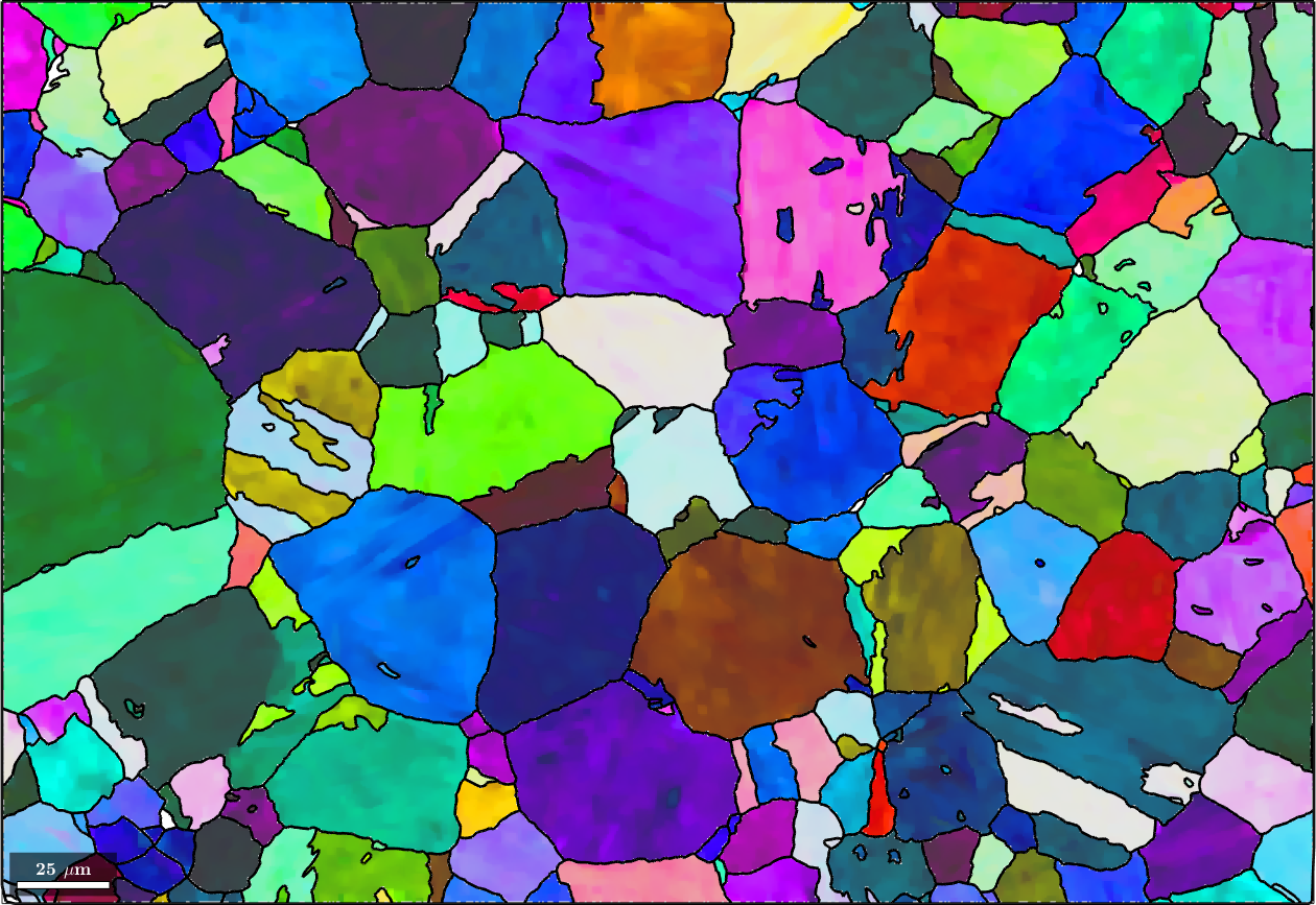
plot(ebsd('Iron bcc'),ebsd('Iron bcc').orientations,'figSize','large')
hold on
plot(grains.boundary,'linewidth',2)
hold off

ebsd = EBSD
 
 Phase  Orientations         Mineral         Color  Symmetry  Crystal reference frame
     0   92415 (27%)      notIndexed                                                 
     1  251187 (73%)  Iron bcc (old)  LightSkyBlue       432                         
 
 Properties: bands, bc, bs, error, mad, reliabilityindex
 Scan unit : um
 X x Y x Z : [0 353] x [0 242] x [0 0]
 Normal vector: (0,0,1)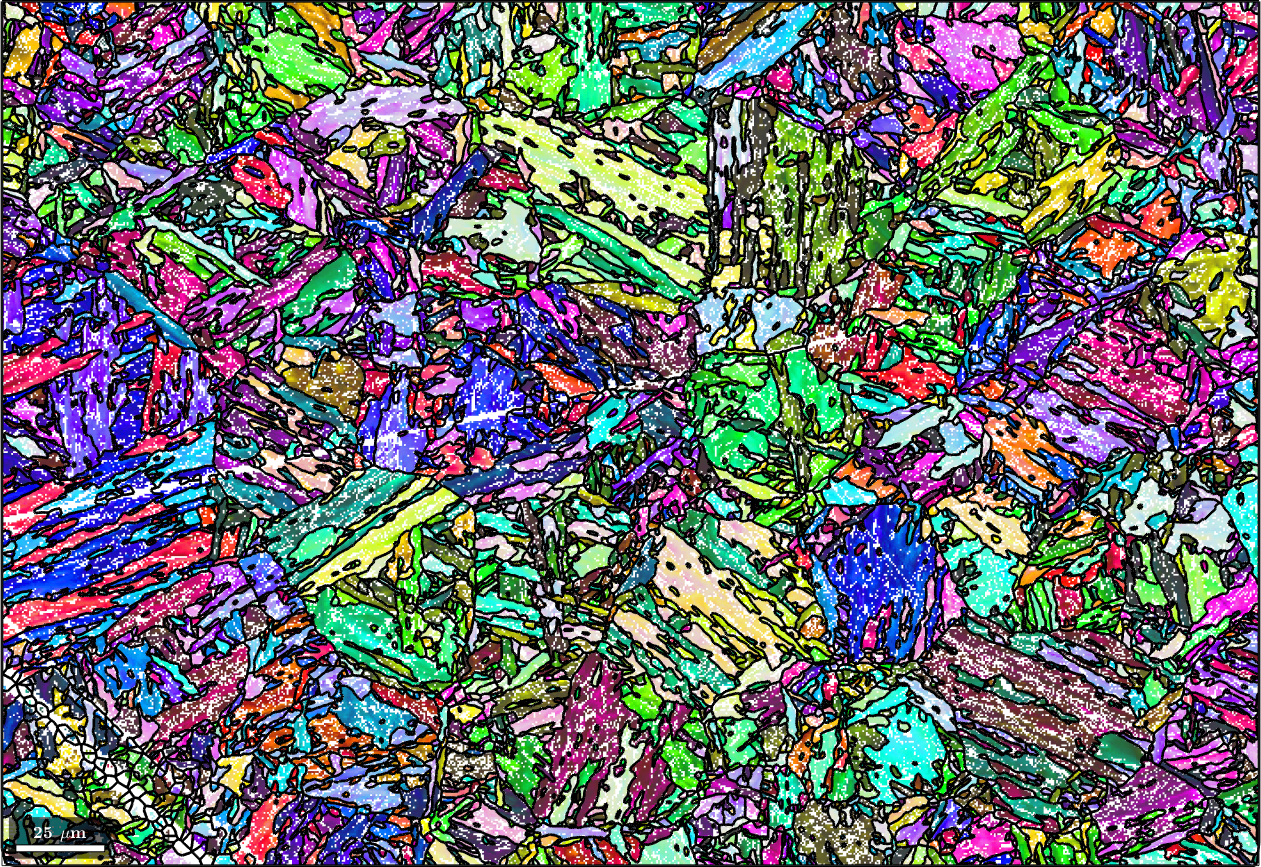

Setting up the parent grain reconstructor

Grain reconstruction is guided in MTEX by a variable of type parentGrainReconstructor. During the reconstruction process this class keeps track about the relationship between the measured child grains and the recovered parent grains.

% set up the job
job = parentGrainReconstructor(ebsd,grains);

The parentGrainReconstructor guesses from the EBSD data what is the parent and what is the child phase. If this guess is not correct it might be specified explicitly by defining an initial guess for the parent to child orientation relationship first and passing it as a third argument to parentGrainReconstructor. Here we define this initial guess separately as the Kurdjumov Sachs orientation relationship

% initial guess for the parent to child orientation relationship
job.p2c = orientation.KurdjumovSachs(job.csParent, job.csChild)

job = parentGrainReconstructor
 
 phase   mineral         symmetry  grains  area  reconstructed
 parent  Iron fcc        432       0       0%    0%           
 child   Iron bcc (old)  432       10641   100%               
 
 OR: (111) || (011)   [10-1] || [11-1]
   c2c fit: 2.5°, 3.5°, 4.4°, 5.3° (quintiles)

The output of the variable job tells us the amount of parent and child grains as well as the percentage of already recovered parent grains. Furthermore, it displays how well the current guess of the parent to child orientation relationship fits the child to child misorientations within our data. In our sample data set this fit is described by the 4 quintiles 2.5°, 3.5°, 4.5° and 5.5°.

Optimizing the parent child orientation relationship

It is well known that the phase transformation from austenite to martensite is not described by a fixed orientation relationship. In fact, the actual orientation relationship needs to be determined for each sample individually. Here, we used the iterative method proposed by Tuomo Nyyssönen and implemented in the function calcParent2Child that starts at our initial guess of the orientation relation ship and iterates towards a more optimal orientation relationship.

close all
histogram(job.calcGBFit./degree,'BinMethod','sqrt')
xlabel('disorientation angle')

job.calcParent2Child

ans = parentGrainReconstructor
 
 phase   mineral         symmetry  grains  area  reconstructed
 parent  Iron fcc        432       0       0%    0%           
 child   Iron bcc (old)  432       10641   100%               
 
 OR: (346.1°,9°,58°)
   c2c fit: 1.3°, 1.8°, 2.2°, 2.9° (quintiles)
   closest ideal OR: (111) || (011)   [1-10] || [100] fit: 2.5°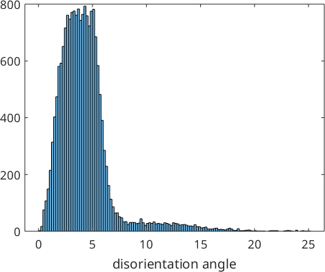

We observe that the optimized parent to child orientation relationship is 2.3° off the initial Kurdjumov Sachs orientation relationship and reduced the first quintil of the misfit with the child to child misorientations to 1.5°. These misfits are stored by the command calcParent2Child in the variable job.fit. In fact, the algorithm assumes that the majority of all boundary misorientations are child to child misorientations and finds the parent to child orientations relationship by minimizing this misfit. The following histogram displays the distribution of the misfit over all grain to grain misorientations.

hold on
histogram(job.calcGBFit./degree,'BinMethod','sqrt')
hold off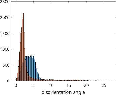

We may explicitly compute the misfit for all child to child boundaries using the command calcGBFit. Beside the list fit it returns also the list of grain pairs for which these fits have been computed. Using the command selectByGrainId we can find the corresponding boundary segments and colorize them according to this misfit. In the code below we go one step further and adjust the transparency as a function of the misfit.

% compute the misfit for all child to child grain neighbors
[fit,c2cPairs] = job.calcGBFit;

% select grain boundary segments by grain ids
[gB,pairId] = job.grains.boundary.selectByGrainId(c2cPairs);

% plot the child phase
plot(ebsd('Iron bcc'),ebsd('Iron bcc').orientations,'figSize','large','faceAlpha',0.5)

% and on top of it the boundaries colorized by the misfit
hold on;
% scale fit between 0 and 1 - required for |edgeAlpha|
plot(gB, 'edgeAlpha', (fit(pairId) ./ degree - 2.5)./2 ,'linewidth',2);
hold off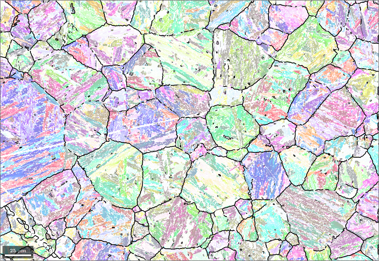

Variant Graph based parent grain reconstruction

Next we set up the variant graph where the nodes are the potential parent orientations of each child grain and the edges describe neighboring grains that have compatible potential parent orientations. This graph is computed by the function calcVariantGraph. The edge weights are computed from the misfit between the potential parent orientations using a cumulative Gaussian distribution with the mean value 'threshold' which describes the misfit at which the probability is exactly 50 percent and the standard deviation 'tolerance'.

job.calcVariantGraph('threshold',3.5*degree,'tolerance',2.5*degree)

ans = parentGrainReconstructor
 
 phase   mineral         symmetry  grains  area  reconstructed
 parent  Iron fcc        432       0       0%    0%           
 child   Iron bcc (old)  432       10641   100%               
 
 OR: (346.1°,9°,58°)
   c2c fit: 1.3°, 1.7°, 2.2°, 3° (quintiles)
   closest ideal OR: (111) || (011)   [1-10] || [100] fit: 2.5°
 
 variant graph: 474481 entries

For large maps it can be useful to perform the segmentation in a two step process, where in the in the first step similarly oriented variants are reconstructed as one variants and only separated in a second step. This can be accomplished by the commands

job.calcVariantGraph('threshold',2.5*degree,'tolerance',2.5*degree,'mergeSimilar')
job.clusterVariantGraph
job.calcVariantGraph('threshold',2.5*degree,'tolerance',2.5*degree)

The next step is to cluster the variant graph into components. This is done by the command clusterVariantGraph.

job.clusterVariantGraph('includeSimilar')

ans = parentGrainReconstructor
 
 phase   mineral         symmetry  grains  area  reconstructed
 parent  Iron fcc        432       0       0%    0%           
 child   Iron bcc (old)  432       10641   100%               
 
 OR: (346.1°,9°,58°)
   c2c fit: 1.3°, 1.8°, 2.2°, 2.9° (quintiles)
   closest ideal OR: (111) || (011)   [1-10] || [100] fit: 2.5°
 
 votes: 10641 x 1
   probabilities: 100%, 100%, 99%, 97% (quintiles)

As a result a table of votes job.votes is generated. More specifically, job.votes.prob is a matrix that contains in row job.votes.prob(i,:) the probabilities of the i-th child grain to have a specific parent orientation. Accordingly, we can plot the probability of the best fit for each grain by

plot(job.grains,job.votes.prob(:,1))
mtexColorbar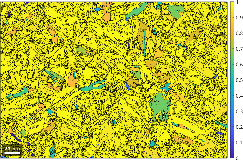

We observe many child grains where the algorithm is sure about the parent orientation and some child grains where the probability is close to 50 percent. This is an indication that there are a least two potential parent orientations which are similarly likely. In many cases these potential parent orientations are in a twinning relationship.

Lets reconstruct all parent orientations where the probability is above 50 percent.

job.calcParentFromVote('minProb',0.5)

% plot the result
plot(job.parentGrains,job.parentGrains.meanOrientation)

ans = parentGrainReconstructor
 
 phase   mineral         symmetry  grains  area   reconstructed
 parent  Iron fcc        432       10558   99%    99%          
 child   Iron bcc (old)  432       83      0.58%               
 
 OR: (346.1°,9°,58°)
   p2c fit: 2.4°, 5°, 9.5°, 19° (quintiles)
   c2c fit: 1.8°, 2.1°, 2.8°, 4° (quintiles)
   closest ideal OR: (111) || (011)   [1-10] || [100] fit: 2.5°
 
 votes: 83 x 1
   probabilities: 0%, 0%, 0%, 0% (quintiles)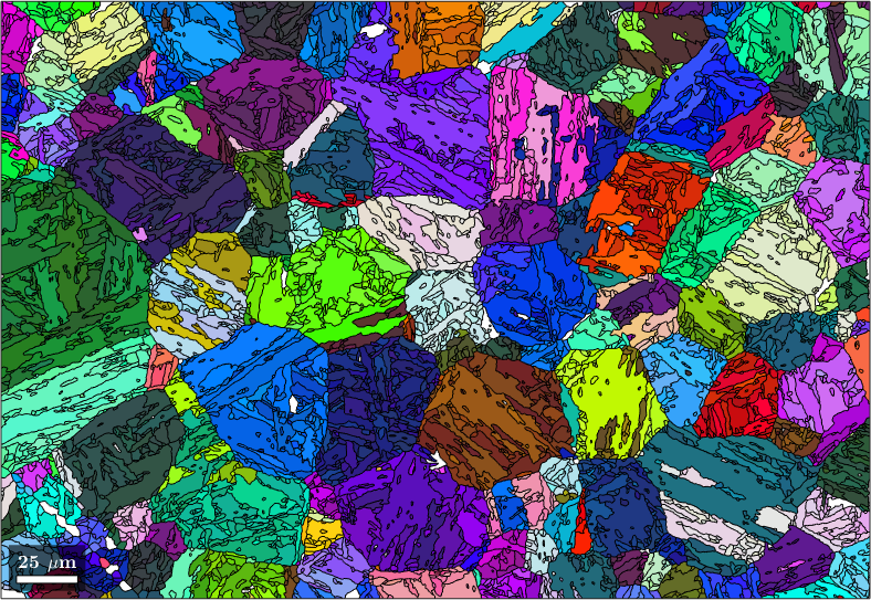

From here we have different possibilities to continue. One possibility is to reconstruct the remaining parent orientations manually. To this end one can use the the command job.selectInteractive. This allow to click any grain and to change its parent orientation into one of the potential parent orientations.

job.selectInteractive

A second way would be to rerun the variant graph approach above a second time but with relaxed settings, i.e., with a lower probability. A third way is to use the command job.calcGBVotes to compute votes for potential parent orientations from the surrounding already reconstructed parent grains.

% compute the votes
job.calcGBVotes('p2c','reconsiderAll','threshold',3*degree,'tolerance',1.5*degree)

% assign parent orientations according to the votes
job.calcParentFromVote

% plot the result
plot(job.parentGrains,job.parentGrains.meanOrientation)

ans = parentGrainReconstructor
 
 phase   mineral         symmetry  grains  area   reconstructed
 parent  Iron fcc        432       10558   99%    99%          
 child   Iron bcc (old)  432       83      0.58%               
 
 OR: (346.1°,9°,58°)
   p2c fit: 2.4°, 5°, 9.5°, 19° (quintiles)
   c2c fit: 1.8°, 2.1°, 2.8°, 4° (quintiles)
   closest ideal OR: (111) || (011)   [1-10] || [100] fit: 2.5°
 
 votes: 10347 x 1
   probabilities: 99%, 93%, 79%, 61% (quintiles)
 
 
ans = parentGrainReconstructor
 
 phase   mineral         symmetry  grains  area   reconstructed
 parent  Iron fcc        432       10575   100%   99%          
 child   Iron bcc (old)  432       66      0.11%               
 
 OR: (346.1°,9°,58°)
   p2c fit: 6°, 10°, 17°, 22° (quintiles)
   c2c fit: 2.1°, 2.4°, 2.6°, 2.9° (quintiles)
   closest ideal OR: (111) || (011)   [1-10] || [100] fit: 2.5°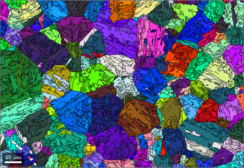

Merge similar grains and inclusions

After the above reconstruction steps most of the child grains have been reverted into parent grains. However, instead of a few big parent grains we still have many small, but similarly oriented parent grains. These can be merged into big parent grains using the command mergeSimilar

% merge grains with similar orientation
job.mergeSimilar('threshold',7.5*degree);

% plot the result
plot(job.parentGrains,job.parentGrains.meanOrientation)

We may be still a bit unsatisfied with the result as the large parent grains contain many poorly indexed inclusions where we failed to assign to a parent orientation. We may use the command mergeInclusions to merge all inclusions with fever pixels then a certain threshold into the surrounding parent grains.

job.mergeInclusions('maxSize',50);

% plot the result
plot(job.parentGrains,job.parentGrains.meanOrientation)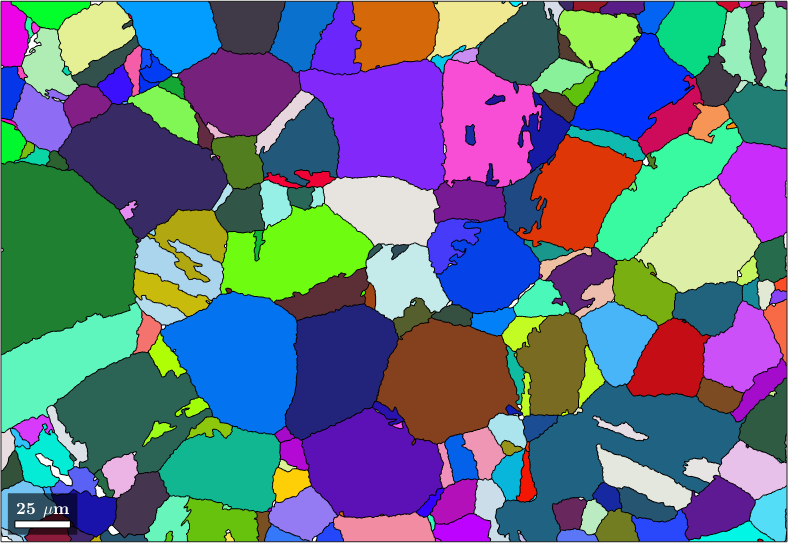

Compute Child Variants

Knowing the parent grain orientations we may compute the variants and packets of each child grain using the command calcVariants. The values are stored with the properties job.transformedGrains.variantId and job.transformedGrains.packetId. The packetId is defined as the closest {111} plane in austenite to the (011) plane in martensite.

job.calcVariants

% associate to each packet id a color and plot
color = ind2color(job.transformedGrains.packetId);
plot(job.transformedGrains,color,'faceAlpha',0.5)

hold on
parentGrains = smooth(job.parentGrains,10);
plot(parentGrains.boundary,'linewidth',3)

% outline a specific parent grain
grainSelected = parentGrains(parentGrains.findByLocation([100,80]));

hold on
plot(grainSelected.boundary,'linewidth',3,'lineColor','w')
hold off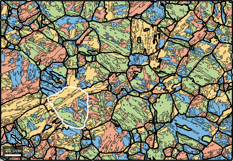

We can also directly identify the child grains belonging to the selected parent grains. Remember that the initial grains are stored in job.grainsPrior and that the vector job.mergeId stores for every initial grain the id of the corresponding parent grain. Combining these two information we do

% identify childs of the selected parent grain
childGrains = job.grainsPrior(job.mergeId == grainSelected.id);

% plot these childs
plot(childGrains,childGrains.meanOrientation)

% and top the parent grain boundary
hold on
plot(grainSelected.boundary,'linewidth',2)
hold off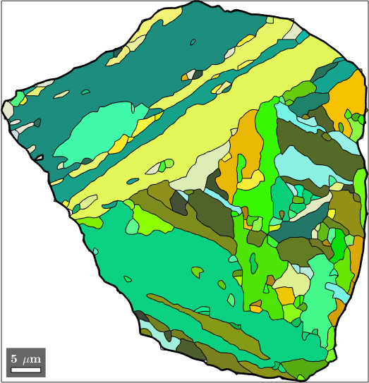

In order to check our parent grain reconstruction we chose the single parent grain outlined in the above map and plot all child variants of its reconstructed parent orientation together with the actually measured child orientations inside the parent grain. In order to compute the variantId and packetId we use the command calcVariantId.

% the measured child orientations that belong to parent grain 279
childOri = job.ebsdPrior(childGrains).orientations;

% the orientation of parent grain 279
parentOri = grainSelected.meanOrientation;

% compute variantIds and packeIds
[variantId, packetId] = calcVariantId(parentOri,childOri,job.p2c);

% colorize child orientations by packetId
color = ind2color(packetId);
plotPDF(childOri,color, Miller(0,0,1,childOri.CS),'MarkerSize',2,'all')

% the positions of the parent (001) directions
hold on
plot(parentOri.symmetrise * Miller(0,0,1,parentOri.CS),'markerSize',10,...
  'marker','s','markerFaceColor','w','MarkerEdgeColor','k','linewidth',2)

% the theoretical child variants
childVariants = variants(job.p2c, parentOri);
plotPDF(childVariants, 'markerFaceColor','none','linewidth',1.5,'markerEdgeColor','k')
hold off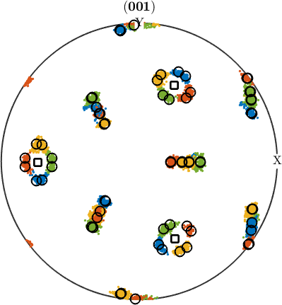

Parent EBSD reconstruction

So far our analysis was at the grain level. However, once parent grain orientations have been computed we may also use them to compute parent orientations of each pixel in our original EBSD map. This is done by the command calcParentEBSD

parentEBSD = job.calcParentEBSD;

% plot the result
plot(parentEBSD('Iron fcc'),parentEBSD('Iron fcc').orientations,'figSize','large')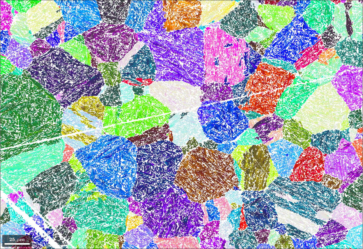

We obtain even a measure parentEBSD.fit for the correspondence between the parent orientation reconstructed from the single pixel and the parent orientation of the grain. Lets visualize this fit

% the fit between ebsd child orientation and the reconstructed parent grain
% orientation
plot(parentEBSD, parentEBSD.fit ./ degree,'figSize','large')
mtexColorbar
setColorRange([0,5])
mtexColorMap('LaboTeX')

hold on
plot(job.grains.boundary,'lineWidth',2)
hold off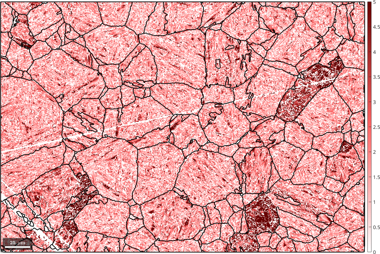

Fill the parent map

Finally, we may apply filtering to the parent map to fill non indexed or not reconstructed pixels. To this end we first run grain reconstruction on the parent map

[parentGrains, parentEBSD.grainId] = calcGrains(parentEBSD('indexed'),'angle',3*degree);

% remove very small grains
parentEBSD(parentGrains(parentGrains.grainSize<10)) = [];

% redo grain reconstruction
[parentGrains, parentEBSD.grainId] = calcGrains(parentEBSD('indexed'),'angle',3*degree);
parentGrains = smooth(parentGrains,10);

plot(ebsd('indexed'),ebsd('indexed').orientations,'figSize','large')

hold on
plot(parentGrains.boundary,'lineWidth',2)
hold off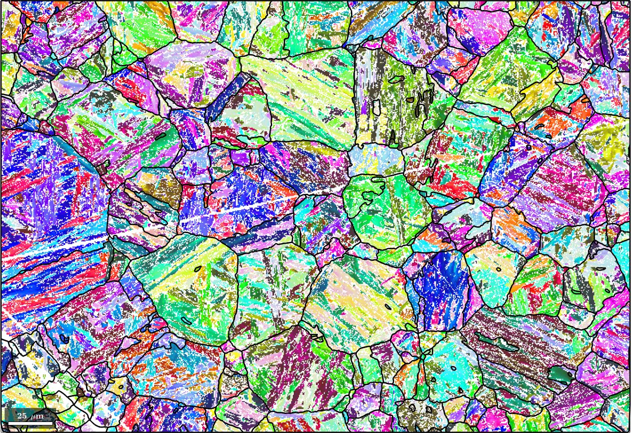

and then use the command smooth to fill the holes in the reconstructed parent map

% fill the holes
F = halfQuadraticFilter;
parentEBSD = smooth(parentEBSD('indexed'),F,'fill',parentGrains);

% plot the parent map
plot(parentEBSD('Iron fcc'),parentEBSD('Iron fcc').orientations,'figSize','large')

% with grain boundaries
hold on
plot(parentGrains.boundary,'lineWidth',2)
hold off