Unimodal ODF Shapes

A unimodal ODF is a normalized peak around one orientation. Its SO(3) kernel sets the profile of that peak: how the density falls with angular distance from the centre.

The halfwidth is the distance at which a kernel has fallen to half its maximum. It is a spread parameter, not normally a cutoff. Matching halfwidths aligns one visible feature, but the tails and peak heights may still differ.

Kernel choice matters when measured orientations are turned into a density; see Density Estimation. It also controls how many harmonic degrees are needed to represent the resulting ODF. Series Expansion introduces that representation and defines its bandwidth.

This page compares kernels for point-centred radial components. Pass an SO3Kernel object to unimodalODF, or use its 'halfwidth' option to select the default de la Vallee Poussin kernel. A fibre ODF is different: current fibreODF accepts an S2Kernel because its density decays across a curve rather than from one orientation.

plottingConvention.default('y↑→x');

psi{1} = SO3AbelPoissonKernel(0.79);
psi{2} = SO3DeLaValleePoussinKernel(13);
psi{3} = SO3BumpKernel(35*degree);
psi{4} = SO3DirichletKernel(3);
psi{5} = SO3vonMisesFisherKernel(7.5);
psi{6} = SO3GaussWeierstrassKernel(0.07);
psi{7} = fibreVonMisesFisherKernel(7.2);
psi{8} = SO3SquareSingularityKernel(0.72);

kernelName = {'Abel-Poisson';'de la Vallee Poussin';'bump';'Dirichlet';...
  'von Mises-Fisher';'Gauss-Weierstrass';'fibre von Mises-Fisher';...
  'square singularity'};

Comparing Halfwidths

The positional arguments above are the native parameters of the eight families. The labelled output converts them to the common halfwidth scale. The values were chosen to span the comparable range from about \(15^\circ\) to \(37^\circ\). The plots below therefore show the difference in shape rather than in width.

halfwidthInDegree = cellfun(@(kernel) kernel.halfwidth./degree,psi);
halfwidthSummary = table(kernelName,halfwidthInDegree(:),...
  'VariableNames',{'kernel','halfwidthInDegree'})

halfwidthSummary =
  8×2 table
              kernel              halfwidthInDegree
    __________________________    _________________
    {'Abel-Poisson'          }          17.45      
    {'de la Vallee Poussin'  }         26.343      
    {'bump'                  }             35      
    {'Dirichlet'             }         36.755      
    {'von Mises-Fisher'      }         24.827      
    {'Gauss-Weierstrass'     }           25.4      
    {'fibre von Mises-Fisher'}          24.92      
    {'square singularity'    }           14.9

Profiles in Orientation Space

Plot each kernel against angular distance from its centre. Every kernel is normalized to mean 1 on orientation space, not to have maximum 1. Narrower profiles can therefore have higher peaks.

close;
figure('position',[100,100,1000,450])
hold on
for i = 1:numel(psi)
  plot(psi{i},'DisplayName',kernelName{i});
end
hold off
xlabel('angle from centre in degree');
ylabel('kernel value');
legend(gca,'show','Location','eastoutside')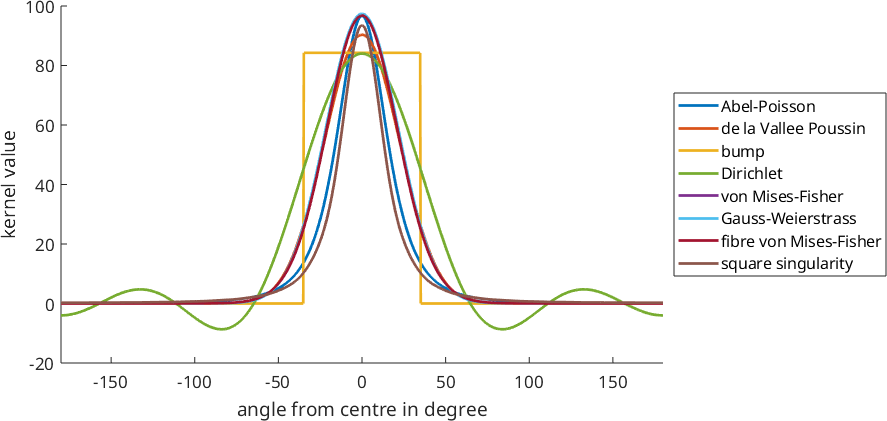

The bump kernel is constant inside its halfwidth and exactly zero outside it. This special cutoff should not be inferred from the meaning of halfwidth in the other families. The Dirichlet kernel oscillates through zero, whereas the smooth families decay with different tails.

A negative kernel is useful for some harmonic calculations, but it is not a probability density. A radial ODF made directly from the Dirichlet kernel can therefore take negative values. The labelled output confirms that this example does.

omega = linspace(0,pi,1000);
dirichletMinimum = min(psi{4}.eval(cos(omega./2)))

dirichletMinimum =
   -8.6660

Projected Profiles in a Pole Figure

A pole figure is the crystallographic Radon transform of an ODF; see Pole Figures of an ODF. Applying that transform to a kernel gives the profile contributed by one radial component to a pole figure peak. This is the curve a measured pole figure peak is compared against.

close;
figure('position',[100,100,1000,450])
hold on
for i = 1:numel(psi)
  plot(psi{i}.radon,'symmetric','DisplayName',kernelName{i},'linewidth',2);
end
hold off
ylim([-5,20])
xlabel('angular distance in degree');
ylabel('projected kernel value');
legend(gca,'show','Location','eastoutside')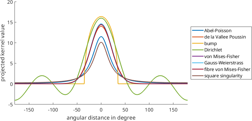

Projection changes the profiles but does not erase their main distinctions. The bump remains compactly supported, and the Dirichlet curve retains negative side lobes. The other curves stay nonnegative but differ in how broadly their pole-figure intensity is spread.

Harmonic Cost

A radial kernel stores one coefficient for every harmonic degree from zero through its bandwidth. Faster coefficient decay permits a lower bandwidth and makes harmonic computations cheaper.

close;
figure('position',[100,100,500,450])
hold on
for i = 1:numel(psi)
  plotSpektra(psi{i},'bandwidth',32,'linewidth',2,...
    'DisplayName',kernelName{i});
end
hold off
xlabel('harmonic degree');
ylabel('radial coefficient');
legend(gca,'show','Location','eastoutside')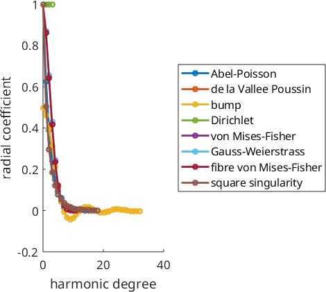

The plot shows only degrees 0 through 32 so that the low-degree decay can be compared. The table reports the full stored bandwidth of each kernel. Bandwidth 10 means degrees 0 through 10 and therefore 11 stored radial coefficients, not 10.

kernelBandwidth = cellfun(@(kernel) kernel.bandwidth,psi);
bandwidthSummary = table(kernelName,kernelBandwidth(:),...
  'VariableNames',{'kernel','bandwidth'})

bandwidthSummary =
  8×2 table
              kernel              bandwidth
    __________________________    _________
    {'Abel-Poisson'          }        16   
    {'de la Vallee Poussin'  }        10   
    {'bump'                  }      1024   
    {'Dirichlet'             }         3   
    {'von Mises-Fisher'      }        11   
    {'Gauss-Weierstrass'     }        11   
    {'fibre von Mises-Fisher'}        11   
    {'square singularity'    }        18

The de la Vallee Poussin kernel ends at bandwidth 10. Both von Mises-Fisher variants and the Gauss-Weierstrass kernel end at 11, whereas the discontinuous bump kernel continues to bandwidth 1024. A sharp edge is expensive in a smooth harmonic basis.

This combination of a finite exact expansion, nonnegative values, and smooth real-space shape is why MTEX uses the de la Vallee Poussin family by default for unimodal ODFs and orientation density estimation.

References

Next

Build point-centred peaks in Radial ODFs and tubular components in Fibre ODFs. The formulas and constructor details for every family are collected in SO(3) Kernels.

References

- Schaeben (1999) derives the de la Vallee Poussin orientation density function and its finite harmonic expansion.
- Hielscher (2013) compares kernel families for density estimation on the rotation group.