Magnetic Anisotropy

Magnetocrystalline anisotropy makes some directions in a crystal easier to magnetize than others. For cubic iron-silicon with a positive first anisotropy constant, the easy directions are the \(\langle100\rangle\) crystal directions.

Texture turns this crystal-scale property into a specimen-scale one. When many easy directions lie near one specimen direction, less energy is needed to align the magnetic moments along it.

This page calculates the average anisotropy energy of a model electrical steel from its orientation distribution function (ODF). It then uses an empirical relation to estimate \(J_{50}\), the magnetic polarization at a field strength of 5000 A/m. The result is a texture-based estimate, not a measured magnetization curve.

Read Orientations first for the orientation action used below. The ODF tutorial introduces model distributions. Dr. Marco Witte, Salzgitter Mannesmann Forschung, contributed the original example in March 2020.

Define the material and its texture

A reference frame is the coordinate system in which data are expressed. Electrical steel is a rolled sheet, so its specimen frame has rolling direction (RD) along x, transverse direction (TD) along y, and sheet normal (ND) along z. The second call states the deliberate plotting convention in which RD points right and TD points up.

specimenFrame.rolling.makeDefault
plottingConvention.default('y↑→x');

% alloy composition in weight percent
siliconContent = 3;
aluminiumContent = 1;

% composition estimates for K1 in 10^4 J/m^3 and Js in T
K1 = 4.77 - 0.21256*siliconContent - 0.03816*aluminiumContent;
Js = 2.162 - 0.043*siliconContent - 0.0625*aluminiumContent;

% cubic crystal symmetry and a Goss-centred model ODF
cs = crystalSymmetry('m-3m');
goss = orientation.goss(cs);
halfwidth = 10*degree;
odf = unimodalODF(goss,'halfwidth',halfwidth);

% draw an equal-weight sample from the ODF
ori = discreteSample(odf,10000);

modelInputs = table(siliconContent,aluminiumContent,halfwidth/degree,...
  length(ori),K1,Js,'VariableNames',...
  {'Si_wtPercent','Al_wtPercent','halfwidth_deg','orientationCount',...
  'K1_1e4_J_per_m3','Js_T'})

modelInputs =
  1×6 table
    Si_wtPercent    Al_wtPercent    halfwidth_deg    orientationCount    K1_1e4_J_per_m3     Js_T 
    ____________    ____________    _____________    ________________    _______________    ______
         3               1               10               10000              4.0942         1.9705

Read the texture before calculating the property

An ODF is a material-volume density over crystal orientations. This model concentrates that density within a 10 degree halfwidth of Goss.

A Goss orientation is \((110)[001]\): the \((110)\) plane lies in the sheet and \([001]\) lies along RD. The pole figure shows where the cubic \(\{100\}\) easy directions occur in the specimen. Its colour scale is in multiples of a random distribution (mrd).

plotPDF(odf,Miller(1,0,0,cs),'antipodal','contourf');
mtexColorbar('title','pole density (mrd)');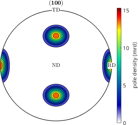

One \(\{100\}\) pole lies at RD, and appears at both the left and the right edge because the plot is antipodal. The other two easy axes project halfway between TD and ND. All three peak at the same density, since the three \(\langle100\rangle\) directions are symmetrically equivalent. A field along RD is therefore close to an easy axis for most orientations, while a field along TD lies between easy axes.

Evaluate directions in the sheet plane

The field turns from RD to TD in 5 degree steps. Each orientation maps crystal coordinates into specimen coordinates, so its inverse maps the specimen field direction into the crystal frame. The code operates on all 10000 sampled orientations at once; only the list of field directions needs a loop.

fieldAngle = 0:5:90;
anisotropyEnergy = zeros(length(fieldAngle),length(ori));

% three separate cubic axes used by the energy expression
h100 = Miller(1,0,0,cs);
h010 = Miller(0,1,0,cs);
h001 = Miller(0,0,1,cs);

for k = 1:length(fieldAngle)

  % express the specimen field direction in every crystal frame
  fieldSpecimen = rotation.byAxisAngle(zvector,...
    fieldAngle(k)*degree) * xvector;
  fieldCrystal = inv(ori) * fieldSpecimen;

  % direction cosines with the three cubic easy axes
  alpha1 = dot(h100,fieldCrystal,'noSymmetry');
  alpha2 = dot(h010,fieldCrystal,'noSymmetry');
  alpha3 = dot(h001,fieldCrystal,'noSymmetry');

  % first-order cubic magnetocrystalline anisotropy energy density
  anisotropyEnergy(k,:) = K1*(alpha1.^2.*alpha2.^2 + ...
    alpha2.^2.*alpha3.^2 + alpha1.^2.*alpha3.^2);

end

Average the texture and estimate J50

The arithmetic mean approximates the ODF-weighted material-volume average because discreteSample drew equal-weight orientations from the ODF. Yonamine et al. fitted the second line below to electrical-steel measurements.

meanEnergy = mean(anisotropyEnergy,2);
predictedJ50 = Js*(1-0.19*meanEnergy);

selectedDirections = [1,10,12,19];
directionalResults = table(fieldAngle(selectedDirections).',...
  round(meanEnergy(selectedDirections),4),...
  round(predictedJ50(selectedDirections),4),...
  'VariableNames',{'angleFromRD_deg','meanEnergy_1e4_J_per_m3',...
  'predictedJ50_T'})

directionalResults =
  4×3 table
    angleFromRD_deg    meanEnergy_1e4_J_per_m3    predictedJ50_T
    _______________    _______________________    ______________
           0                   0.1611                 1.9102    
          45                   1.1871                 1.5261    
          55                   1.2581                 1.4995    
          90                   0.9845                 1.6019

At RD the mean energy is 0.1628 in units of \(10^4\) J/m\(^3\), and the predicted \(J_{50}\) is 1.9095 T. The sampled maximum occurs at 55 degrees: 1.2566 in the same energy units and 1.5 T. Toward TD the energy falls to 0.9833 and the predicted polarization recovers to 1.6024 T.

Plot the directional result

figure;
subplot(2,1,1);
plot(fieldAngle,meanEnergy,'LineWidth',2);
xlabel('angle from RD (degree)');
ylabel('mean energy (10^4 J/m^3)');
grid on;

subplot(2,1,2);
plot(fieldAngle,predictedJ50,'LineWidth',2);
xlabel('angle from RD (degree)');
ylabel('predicted J_{50} (T)');
grid on;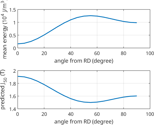

RD has the lowest mean energy and the highest predicted \(J_{50}\). The energy rises as the field leaves the Goss \([001]\) direction and reaches a broad maximum between RD and TD. The lower panel is the inverse of the upper trend because the empirical relation is linear in mean energy.

Why noSymmetry is required

The first-order energy density for a cubic crystal is

\[ E_a=K_1\left(\alpha_1^2\alpha_2^2+ \alpha_2^2\alpha_3^2+\alpha_3^2\alpha_1^2\right), \]

where \(\alpha_1\), \(\alpha_2\), and \(\alpha_3\) are the direction cosines between the magnetization and the three crystal axes. The expression is invariant when cubic symmetry permutes or reverses those axes.

The three cosines still have to be evaluated separately. Without 'noSymmetry', dot compares a direction with symmetrically equivalent Miller directions and returns the best match. That would replace the three components required by the equation with three symmetry-reduced comparisons.

What this estimate leaves out

This page evaluates the quartic energy law directly rather than creating an MTEX tensor object. The orientation and ODF supply the frame changes and the texture average.

The model retains composition, crystal anisotropy, and texture. It omits domain-wall motion, demagnetizing fields, stress, and magnetostriction. Grain size, defects, and cutting damage are also absent. Those effects can change a real magnetization curve even when the ODF is unchanged.

The \(J_{50}\) correlation was fitted to non-oriented electrical steels. The sharply Goss-centred ODF used here makes the directional mechanism easy to see, but it does not validate the fit for a commercial grain-oriented grade. Compare an estimate with measurements made under a stated standard before using it as a material property.

Next

Tensor Averages develops orientation averaging for typed elastic tensors and distinguishes Voigt, Reuss, and Hill estimates. the ODF tutorial shows how a model or measured ODF is constructed. Elasticity continues from texture to directional properties represented by rank four tensors.

Further reading