Triple Points

A triple point is a junction where exactly three grain boundary segments meet and separate three distinct real grains. It is therefore a strict subset of the junctions in a boundary network. An endpoint at the scan rim is a junction, for example, but it is not a triple point.

MTEX computes triple points automatically during grain reconstruction. They are available from a grain list through grains.triplePoints, just as the boundary segments are available through grains.boundary. The result is a triplePointList.

A square measurement grid can also produce vertices where four boundary segments meet. When analysing triple points, it is a good idea to pass 'removeQuadruplePoints' to calcGrains. This converts each ambiguous quadruple point into two triple points. Quadruple Points explains the resulting topology.

This page assumes that the map has already been divided into grains as in Grain Reconstruction. Select Grain Boundaries introduces boundary-list indexing, and Boundary Misorientations explains the disorientations used below.

close all;

% load the example map in its specimen plotting frame
plottingConvention.default('y↑→x');
mtexdata small silent

% reconstruct the grains and resolve quadruple points
grains = calcGrains(ebsd,'removeQuadruplePoints','alpha',5);

% smooth the pixel staircase while keeping junctions fixed
grains = smoothBoundary(grains,2);

% draw the grains and overlay all triple points
plot(grains);
tP = grains.triplePoints
hold on
plot(tP,'color','b','linewidth',2)
hold off

tP = triplePointList (y↑→x)
 
 points   mineral 1   mineral 2   mineral 3
     14  Forsterite  Forsterite  Forsterite
      7  Forsterite  Forsterite   Enstatite
      4  Forsterite   Enstatite   Enstatite
      9  Forsterite  Forsterite    Diopside
     18  Forsterite   Enstatite    Diopside
      4  Forsterite    Diopside    Diopside
      2   Enstatite   Enstatite    Diopside
      1   Enstatite    Diopside    Diopside
     11    Diopside    Diopside    Diopside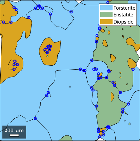

The blue circles lie only where three real grains meet. They do not mark loose ends at the map rim or every crossing in the boundary network.

Select by phase

Phase names select triple points by the phases of their three adjacent grains. Repeating a name requests that multiplicity; the names do not assign an order to the three sides. One name therefore means at least one adjacent forsterite grain.

tP('Forsterite')

ans = triplePointList (y↑→x)
 
 points   mineral 1   mineral 2   mineral 3
     14  Forsterite  Forsterite  Forsterite
      7  Forsterite  Forsterite   Enstatite
      4  Forsterite   Enstatite   Enstatite
      9  Forsterite  Forsterite    Diopside
     18  Forsterite   Enstatite    Diopside
      4  Forsterite    Diopside    Diopside

Repeating the name selects points with at least two adjacent forsterite grains.

tP('Forsterite','Forsterite')

ans = triplePointList (y↑→x)
 
 points   mineral 1   mineral 2   mineral 3
     14  Forsterite  Forsterite  Forsterite
      7  Forsterite  Forsterite   Enstatite
      9  Forsterite  Forsterite    Diopside

Three repeated names restrict the selection to inner diopside triple points, where all three adjacent grains are diopside.

hold on
plot(tP('Diopside','Diopside','Diopside'),...
  'displayName','Di-Di-Di','color','darkred','linewidth',2)
hold off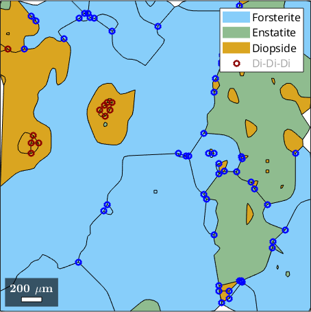

The dark-red circles are a subset of the blue points. Their locations show where the diopside boundary network branches entirely within that phase.

Select by grain

A triple point also belongs to each of its three adjacent grains. A grain selection therefore returns the points on the boundary of that grain.

% find the list position of the largest grain
[~,largestIndex] = max(grains.area);

% extract and plot the triple points of that grain
tP_largest = grains(largestIndex).triplePoints;
plot(grains(largestIndex),'FaceColor',[0.2 0.8 0.8],...
  'displayName','largest grain');
hold on
plot(grains.boundary)
plot(tP_largest,'color','r','linewidth',2)
hold off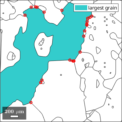

The red circles occur only where the cyan grain meets two other grains. The black network supplies the surrounding context that a grain outline alone would hide.

Select through grain boundaries

Triple points are also stored with a grainBoundary selection. Here the eligible segments are first restricted to forsterite--forsterite boundaries, so every disorientation has one consistent phase pair.

% all forsterite--forsterite boundary segments
gB_Fo = grains.boundary('Forsterite','Forsterite')

% retain segments whose disorientation angle is larger than 60 degrees
gB_large = gB_Fo(gB_Fo.misorientation.angle > 60*degree)

% plot those segments and every triple point incident to at least one of them
plot(grains)
hold on
plot(gB_large,'linewidth',2,'linecolor','w')
plot(gB_large.triplePoints,'color','m','linewidth',2)
hold off

gB_Fo = grainBoundary (y↑→x)
 
 Segments    length   mineral 1   mineral 2
      220  10207 µm  Forsterite  Forsterite
 
gB_large = grainBoundary (y↑→x)
 
 Segments   length   mineral 1   mineral 2
       49  2228 µm  Forsterite  Forsterite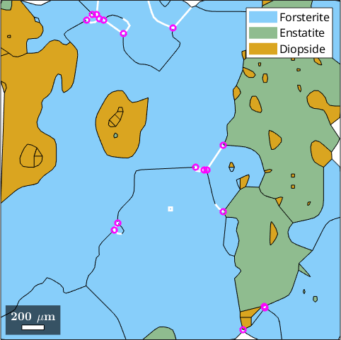

White marks the selected high-angle segments. A magenta circle means that at least one selected segment reaches that point; it does not mean that all three incident segments exceed 60 degrees.

Boundary segments at a triple point

The boundaryId property has one row per triple point and three columns for its incident segments. These values index the complete boundary list from which the triple points came. Here all three neighbouring grains are first restricted to forsterite.

% select forsterite--forsterite--forsterite triple points
tP_Fo = grains.triplePoints('Fo','Fo','Fo');

% extract the three incident boundary segments for every selected point
gB = grains.boundary(tP_Fo.boundaryId);

% plot the incident segments
plot(grains)
hold on
plot(gB,'lineColor','w','linewidth',2)
hold off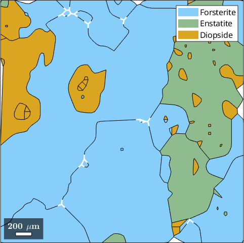

The white three-armed groups are the local boundary neighbourhoods of the selected points. Use tP_Fo.boundaryId(:) when a single list of segments is wanted instead of this point-by-segment arrangement.

Disorientations around the point

The same indexing extracts the disorientation across each incident segment. The displayed object has size \(n \times 3\), where \(n\) is the number of selected triple points.

mori = gB.misorientation

mori = misorientation (Forsterite → Forsterite)
  size: 14 × 3
  antipodal: true

A simple scalar summary is the sum of the three disorientation angles at each point.

sumMisAngle = sum(mori.angle,2);

plot(grains,'figSize','large')
hold on
plot(tP_Fo,sumMisAngle ./ degree,...
  'markerEdgeColor','w','MarkerSize',8)
hold off
mtexColorMap(blue2redColorMap)
setColorRange([80,180])
mtexColorbar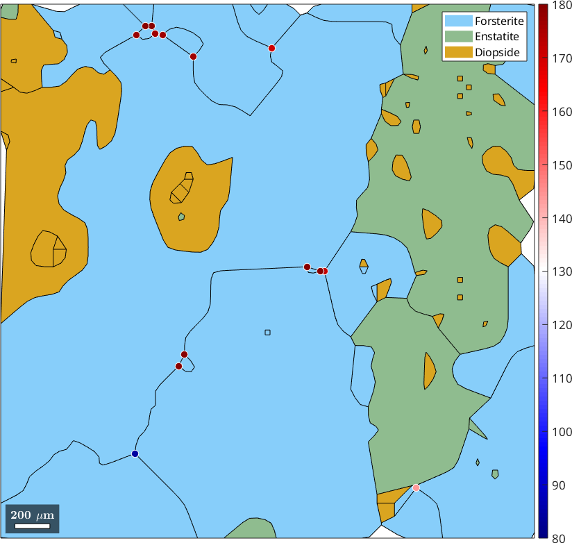

Colour records that angle sum in degrees. The fixed colour range saturates any sum above 180 degrees at its upper colour. This scalar is descriptive, not a crystallographic closure condition. The underlying ordered rotations close around the three grains, but their three minimum disorientation angles do not generally add to a fixed value.

Section angles at triple points

The property tP.angles returns the three angles enclosed by the incident boundary segments. It is an \(n \times 3\) matrix, and each row sums to \(2\pi\). The spread between the largest and smallest angle measures how unequal the three arms appear in this two-dimensional section.

tP = grains.triplePoints;
angleSpread = (max(tP.angles,[],2) - min(tP.angles,[],2)) ./ degree;

plot(grains,'figSize','large')
hold on
plot(tP,angleSpread,'markerEdgeColor','w','MarkerSize',8)
hold off
mtexColorMap LaboTeX
setColorRange([0,180])
mtexColorbar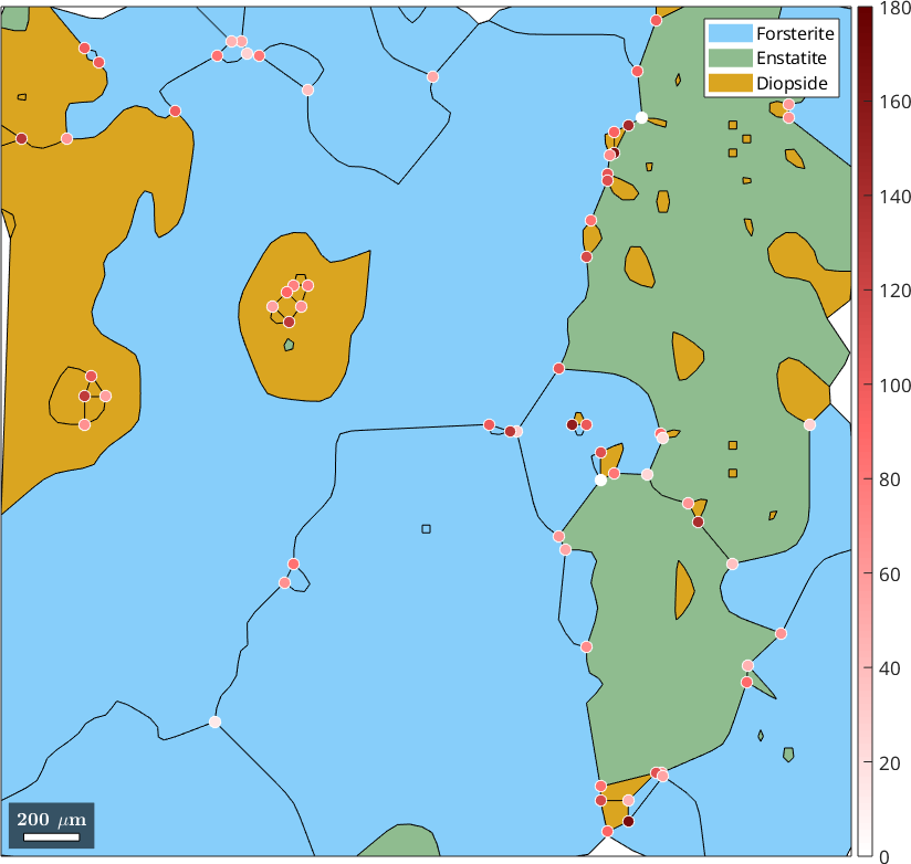

Pale points have three more nearly equal section angles, while dark-red points have a larger angular spread. These are angles between smoothed traces in the section, not the full dihedral angles of three boundary planes in three dimensions.

In a section perpendicular to the three-dimensional junction line, equal, orientation-independent boundary energies at local equilibrium would give three 120 degree angles. Unequal energies, anisotropy, drag, non-equilibrium microstructure, sectioning, and segmentation can all move the observed values away from that ideal. The angle spread must therefore not be read directly as a boundary-energy measurement.

Further reading

Next

Continue with Quadruple Points for the grid ambiguity resolved at reconstruction. CSL Boundaries classifies triple points by the character of their incident boundaries. Merging Grains then shows how selected boundaries alter the grains and their junction network. For full boundary-plane geometry, continue to 3D EBSD. Triple points also supply local orientation evidence in Triple Point Based Reconstruction of parent grains.