Grain Boundaries

From grains to a boundary network

A grain is a phase-homogeneous, spatially connected region of EBSD pixels produced by segmentation. Begin this chapter after Grain Reconstruction has divided a map into those regions.

The interface between two grains often matters as much as either grain. Its character influences how a material fractures and corrodes. It also affects how readily an atom or dislocation crosses the interface.

MTEX represents a grain boundary as short segments. Each segment lies between neighbouring measurements that were assigned to different grains. One grainBoundary object holds the whole segment list, and its methods act across that list. The segments have properties; they are not decoration drawn over the grains.

close all;

% load and crop the example map in its specimen plotting frame
plottingConvention.default('y↑→x');
mtexdata forsterite silent
ebsd = ebsd(inpolygon(ebsd,[5 2 10 5]*10^3));

% reconstruct and smooth the grains
grains = calcGrains(ebsd('indexed'),'angle',10*degree);
grains = smoothBoundary(grains,5);

% display the boundary list
gB = grains.boundary

% draw the grains, boundary network, and strict triple points
plot(grains,'noBoundary','micronbar','off')
hold on
plot(gB,'lineWidth',1.5)
plot(grains.triplePoints,'color','r','MarkerSize',4)
hold off

gB = grainBoundary (y↑→x)
 
 Segments    length   mineral 1   mineral 2
      639  31408 µm  notIndexed  Forsterite
       40   1955 µm  notIndexed   Enstatite
       33   1514 µm  notIndexed    Diopside
     1317  58893 µm  Forsterite  Forsterite
      671  28918 µm  Forsterite   Enstatite
      576  24670 µm  Forsterite    Diopside
       33   1543 µm   Enstatite   Enstatite
      169   7322 µm   Enstatite    Diopside
      111   4561 µm    Diopside    Diopside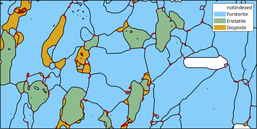

Reading the boundary object and figure

The displayed summary groups the segments by the phases on their two sides. Each row reports a segment count and the total trace length. notIndexed normally denotes pixels whose patterns could not be indexed. In this indexed-only example, a notIndexed side in that table marks the outer scan rim, where no neighbouring grain exists beyond the map.

The coloured regions in the figure are grains, and the black lines are their boundary network. The red markers are triple points. A junction is a vertex where the number of meeting segments is not two. A triple point is a junction where exactly three segments meet and separate three distinct real grains. They are not merely places where two plotted lines cross.

At equilibrium, the angles at a triple point reflect interfacial force balance. That balance depends on the relative energies and their anisotropy. A junction therefore carries information that no single segment does. A two-dimensional section also depends on how the specimen was cut. Its angles are not a direct energy measurement without equilibrium and section-geometry assumptions.

Five macroscopic parameters

Describing a grain boundary completely at a macroscopic scale takes five independent parameters. Three specify the misorientation between the two crystal lattices. Two specify the direction of the interface-plane normal. Boundaries with the same misorientation but different planes are different interfaces and can behave differently.

A polished two-dimensional section supplies four of these five parameters. The crystal orientations give the misorientation, while the boundary trace gives the line where the interface plane meets the section. The inclination of that plane remains unknown, because a trace is consistent with any plane that contains it.

3D EBSD can resolve the plane of an individual interface. From two-dimensional data, Boundary Normal Distribution estimates a population of plane orientations from many traces. It does not recover the missing inclination of every individual segment.

Boundary categories are queries, not new classes

A phase boundary is not a separate type of object in MTEX. It is a grain boundary whose two neighbouring grains differ in phase. Selecting phase boundaries is a query on the same grainBoundary list.

A phase change always separates neighbouring pixels into different grains. For one phase, the usual one-threshold reconstruction separates neighbours whose misorientation exceeds the segmentation angle. Their segments appear in grains.boundary. A two-threshold reconstruction can also preserve lower-angle walls within grains in grains.innerBoundary.

A low-angle boundary is defined by its misorientation angle. A subgrain boundary lies inside a grain. The two populations usually overlap, but they are not synonyms. Subgrain boundaries are real features, commonly dislocation walls, and an analysis of grain outlines alone cannot see them.

Recommended reading order

Follow the order in the chapter contents. Begin with Select. It filters the boundary list by phase, grain, or property. Plot then colours those selected segments by scalar, directional, or full-misorientation data.

Properties introduces two-sided IDs, length, direction, and the network connections of each segment. Read it before Misorientations. That page develops the relationship across a segment and the reference frame of its misorientation axis.

Subgrain Boundaries comes next because it explains the two thresholds used by Twist and Tilt. The latter compares the misorientation axis with the boundary trace, the classic physical distinction between tilt, twist, and mixed character. CSL then introduces coincidence site lattice relationships. At such a relationship, the lattices share some sites. Coincidence is a geometric classification. It does not by itself guarantee a low-energy boundary. Some boundaries with low \(\Sigma\) values and suitable planes are nevertheless especially low in energy.

The geometry route begins with Curvature, which shows why a pixel staircase cannot be interpreted as a smooth interface. Smoothing explains the measurement decision. Smoothing Algorithms compares the filters. Raw staircases corrupt length, direction, and curvature. Smoothing is therefore not cosmetic, but it moves the boundary. The method and smoothing scale are analysis decisions.

Twinning returns to crystallographic character and infers a repeated twin relationship from a real microstructure. Twins are a special boundary population that dominates many materials.

Triple Points and Quadruple Points treat the network junctions. Exact four-way contacts are generally unstable in a physical two-dimensional network. On a square measurement grid they also arise as a digital-connectivity ambiguity during segmentation. An apparent four-way contact may therefore represent two physical triple points that the section or segmentation has placed at the same location.

Intersections treats the network as geometry crossed by a test line. Finish with Distribution, which estimates boundary-plane populations. That page also assumes the kernel-density ideas introduced in Density Estimation.

References

Next

The regions separated here are introduced in Grains, and the lattice relationships across them in Misorientations. Selected relationships created by a solid-state transformation feed into Phase Transitions.

The next top-level chapter is 3D EBSD. Its interface faces supply the inclination that a two-dimensional boundary trace lacks.

References

- A. P. Sutton and R. W. Balluffi, Interfaces in Crystalline Materials, Clarendon Press, 1995. This textbook develops interface structure, thermodynamics, and kinetics.
- F. Bachmann, R. Hielscher, and H. Schaeben, Grain Detection from 2d and 3d EBSD Data - Specification of the MTEX Algorithm, Ultramicroscopy 111 (2011), 1720--1733. This paper derives the reconstructed boundary network.
- A. P. Sutton, E. P. Banks, and A. R. Warwick, The Five-Dimensional Parameter Space of Grain Boundaries, Proceedings of the Royal Society A 471 (2015), 20150442. This paper separates misorientation from plane orientation.
- D. M. Saylor, B. S. El-Dasher, B. L. Adams, and G. S. Rohrer, Measuring the Five-Parameter Grain-Boundary Distribution from Observations of Planar Sections, Metallurgical and Materials Transactions A 35 (2004), 1981--1989.
- G. S. Rohrer, Grain Boundary Energy Anisotropy: A Review, Journal of Materials Science 46 (2011), 5881--5895. This review relates the five parameters and junction geometry to energy.