Misorientations

An orientation maps one crystal frame into the specimen frame. A misorientation maps one crystal frame into another. The specimen frame therefore cancels from the relative relationship.

Changing the specimen frame changes both orientation descriptions together, but it does not change their misorientation. Turn the sample on the stage and every orientation changes, but no misorientation does. This independence is why misorientations carry so much of the physics.

Misorientations describe neighbouring pixels, a pixel relative to its grain mean, crystals across a grain boundary, and crystals in different phases. They quantify orientation gradients and internal grain bending, identify twin relationships, and connect martensite to a possible parent grain.

The example below is a magnesium EBSD map containing extension twins. The grains are reconstructed at a \(5^\circ\) threshold. Their boundaries are coloured by the misorientation angle across them.

plottingConvention.default('y↑→x');
mtexdata twins silent

grains = calcGrains(ebsd('indexed'),'angle',5*degree);
grains = smoothBoundary(grains,5);
gB = grains.boundary('Magnesium','Magnesium');

plot(grains,'FaceColor',[0.92 0.92 0.92],'micronbar','off')
hold on
plot(gB,gB.misorientation.angle./degree,'linewidth',3)
mtexColorbar('title','misorientation angle in degree')
hold off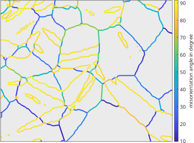

The yellow traces share an angle near \(86^\circ\), while the cooler traces span lower angles. The neutral grain interiors keep orientation colour from being confused with the boundary-angle scale.

This map shows only the angle. It does not yet establish that the yellow boundaries share the same rotation axis or arise from the same mechanism.

From Individual Boundaries to a Population

Plotting the same segment angles as a histogram reveals the repeated relationship directly.

close all
plotAngleDistribution(gB.misorientation,'figSize','small')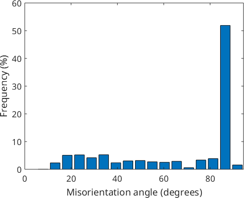

The sharp population near \(86^\circ\) is the signature of the extension twin in this map. A broader population occupies the lower angles.

Each boundary segment contributes one sample, not each neighbouring grain pair. Long boundaries usually have more segments, so the histogram depends on boundary sampling. Interpreting such populations is central to this chapter.

Misorientation, Disorientation, and Symmetry

A crystal has symmetry, so one physical misorientation has many equivalent rotation descriptions. For a cubic crystal there are 24 ways to label the lattice axes on each side, giving up to \(24 \times 24 = 576\) rotations.

Each rotation is a symmetrically equivalent representative of the same misorientation. A disorientation is the particular representative with the smallest rotation angle and an axis in a fundamental sector. A fundamental region is the part of rotation space that keeps exactly one representative of each physical relationship.

When a boundary is called a "60 degree boundary", the quoted value is its disorientation angle. The angle is not the complete misorientation because it says nothing about the rotation axis.

The symmetries on both sides determine the equivalent rotations. The same numerical angle must therefore be compared across phases with care.

A further ambiguity occurs at a same-phase grain boundary. Neither side is intrinsically first. Reversing their order replaces the misorientation by its inverse.

Grain exchange symmetry identifies those two descriptions. Include it when boundary misorientations are counted into a distribution. Otherwise one boundary can appear as two different relationships.

Angle, Axis, and Boundary Plane

A rotation needs an angle and an axis. Different misorientations can have the same angle, so the histogram above cannot identify a twin law by itself. The complete relationship must be compared before a mechanism is assigned.

An axis also needs a reference frame. It may be expressed as a direction in either crystal frame or in the specimen frame, and those questions are not interchangeable.

A misorientation is still not a complete grain-boundary description. It supplies three rotational degrees of freedom; the interface-plane normal supplies two more. The Grain Boundaries chapter adds that spatial information.

Where to Start

Begin with Orientations as Coordinate Transforms if composition order is unfamiliar. The EBSD examples also use grain reconstruction. The distribution pages assume kernel density estimation.

The recommended reading order follows the chapter contents:

The misorientation distribution function, or MDF, plays the same role for misorientations that the ODF plays for orientations. Its angle and axis distributions are often easier to read, but neither retains their coupling.

Compare a measured boundary distribution with its texture-dependent uncorrelated distribution. Also compare it with the symmetry-only random baseline. These tests ask whether texture or rotation-space geometry explains a population. A difference does not prove a physical mechanism.

References

Next

The next documentation chapter introduces orientation distribution functions. They provide the texture-dependent reference used later in this chapter.

For spatial applications, continue to Grain Boundaries. Its CSL and detailed twinning analyses add boundary geometry to the relative rotations introduced here. Parent-to-child misorientations drive Phase Transitions.

Pixel-to-pixel and pixel-to-grain mean misorientations continue in Kernel Average Misorientation and Grain Orientation Parameters.

Return to Orientations when the underlying crystal-to-specimen maps or their reference frames need review.

References

- A. Morawiec, Orientations and Rotations: Computations in Crystallographic Textures, Springer, 2004. This book develops rotation space, symmetry, and misorientation distributions.
- J.K. Mackenzie, Second Paper on Statistics Associated with the Random Disorientation of Cubes, Biometrika 45 (1958), 229--240. This paper derives the cubic random baseline.
- J.W. Christian and S. Mahajan, Deformation Twinning, Progress in Materials Science 39 (1995), 1--157. This review covers twin modes and their crystallography.
- A.P. Sutton, E.P. Banks, and A.R. Warwick, The Five-Dimensional Parameter Space of Grain Boundaries, Proceedings of the Royal Society A 471 (2015), 20150442. This paper separates misorientation from boundary-plane orientation.
- ISO 24173:2024, Microbeam analysis -- Guidelines for orientation measurement using electron backscatter diffraction. This standard addresses reproducible EBSD measurements.