Phase Transitions

During a solid-state phase transition, new crystals do not appear at random orientations. The old lattice remains while the new one forms, so a low-energy change keeps as many atomic planes and directions aligned as possible. The result is the fixed angular relation between parent and child lattices developed in Fitting the Orientation Relationship. The same OR applies wherever that transformation occurs.

Symmetry turns that one relation into several possible child orientations. A parent lattice with 24 proper rotations can satisfy the same relation in distinct ways. These possibilities are the variants defined on the fitting page, and one parent grain commonly transforms into several variants at once.

plottingConvention.default('y↑→x');

See the variants from one parent

The example uses a Kurdjumov-Sachs (KS) relationship between parent austenite and child ferrite. The pole figure shows the child orientations that one parent orientation can produce.

csParent = crystalSymmetry('m-3m',[3.65 3.65 3.65],...
  'mineral','Austenite');
csChild = crystalSymmetry('m-3m',[2.87 2.87 2.87],...
  'mineral','Ferrite');

p2c = orientation.KurdjumovSachs(csParent,csChild);

oriParent = orientation.byEuler(0,0,0,csParent);
oriChild = variants(p2c,oriParent);

plotPDF(oriChild,Miller(0,0,1,csChild),...
  'MarkerSize',8,'figSize','small')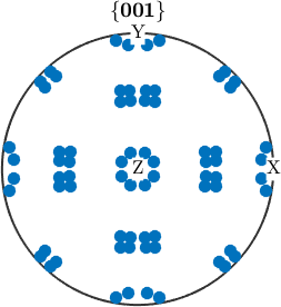

Notice the 24 variants produced from one parent orientation. Each contributes three symmetrically equivalent (001) poles, so the figure carries 72 pole positions. KS gives 24 variants, whereas the Nishiyama-Wassermann relationship gives 12. A real steel may follow neither ideal relationship exactly. The measured data must determine which relationship and variants are present.

Read the transformation backwards

In many experiments only the child phase survives to be measured. Examples include martensite, ferrite, and alpha titanium. The former parent-grain structure may nevertheless control the material's properties, so the metallurgist wants to recover it.

Parent grain reconstruction solves this inverse problem. Children from one parent are variants of a common parent orientation. Neighbouring child grains that are mutually consistent with the OR can therefore be traced back to one parent.

The reconstruction has two steps that must remain distinct. First, each child grain is transformed individually to a candidate parent orientation. Second, neighbouring candidates with compatible parent orientations are merged into one parent-grain footprint.

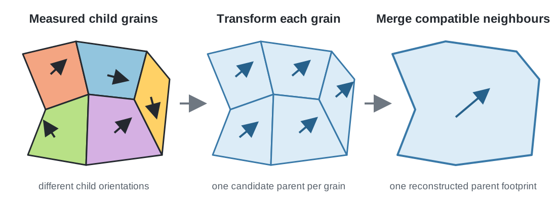
The middle panel keeps the child-grain footprints separate while their candidate parent orientations align. Only the final merge removes the internal boundaries and creates the reconstructed parent grain.

A single child grain is compatible with several possible parents. Choosing among them requires evidence from neighbouring grains. Reconstruction methods are therefore graph problems rather than independent calculations for each grain.

Relate variants, packets, and Bain groups

A packet is a coarse grouping of variants that share the same habit plane. For KS-type martensite, this is the parent {111} plane to which a variant's child lattice aligns.

A Bain group is a coarse grouping by Bain correspondence. It records which parent {001} cube-axis plane a variant's child lattice aligns to.

Packet and Bain group are independent classifications of the same variants. A variant belongs to one packet and one Bain group, but neither grouping is a subdivision of the other.

Follow the chapter

Begin with Parent and Child Variants for the forward and inverse variant calculations. Martensite Variants then fits a measured OR and assigns variant, packet, and Bain group IDs.

Two complete reconstructions follow. Parent Beta Phase Reconstruction treats titanium, and Parent Austenite Reconstruction treats steel. Start with the material system closest to your own.

Transformation Texture asks the forward question: given a parent texture and an OR, what child texture results?

The remaining pages expose the reconstruction algorithms. Grain Graph Based Reconstruction uses grain-to-grain compatibility. Triple Point Based Reconstruction uses the stronger constraint where three grains meet. Low Level Reconstruction and Low Level Reconstruction 2 show the individual steps for cases the automatic workflow handles poorly.

The chapter ends with Fitting the Orientation Relationship, which explains the fitting objective and its local and global solutions. In an applied reconstruction, fit the material's OR before committing parent variants; the worked reconstruction pages demonstrate that sequence first. A measured OR may differ from a textbook relation enough to change the reconstructed result visibly.

Connect to the prerequisite chapters

An OR is a misorientation with the additional parent and child phase symmetries. Reconstructed grains use the segmentation model introduced in Grains. Their measurements and maps come from EBSD Analysis.

References

Next

Continue with Parent and Child Variants to compute the child variants of one parent and the candidate parents of one child.

References

- F. Niessen, T. Nyyssönen, A. A. Gazder, and R. Hielscher, Parent grain reconstruction from partially or fully transformed microstructures in MTEX, Journal of Applied Crystallography 55 (2022), 180-194, defines the generic MTEX reconstruction framework and its transform-and-merge workflow.
- S. Morito, X. Huang, T. Furuhara, T. Maki, and N. Hansen, The morphology and crystallography of lath martensite in alloy steels, Acta Materialia 54 (2006), 5323-5331, gives the variant and packet crystallography summarized here.