Grain Graph Based Parent Grain Reconstrution

Grain Graph Based Parent Grain Reconstrution edit page

This script demonstrates the grain graph approach to parent phase reconstruction in a martensitic material. The methods are described in more detail in the publications

Parent grain reconstruction from partially or fully transformed microstructures in MTEX, J. Appl. Cryst. 55, 2022.
Crystallography, Morphology, and Martensite Transformation of Prior Austenite in Intercritically Annealed High-Aluminum Steel

We shall use the following sample data set.

% load the data
mtexdata martensite
plotx2east

% grain reconstruction
[grains,ebsd.grainId] = calcGrains(ebsd('indexed'), 'angle', 3*degree,'minPixel',2);
grains = smooth(grains,5);

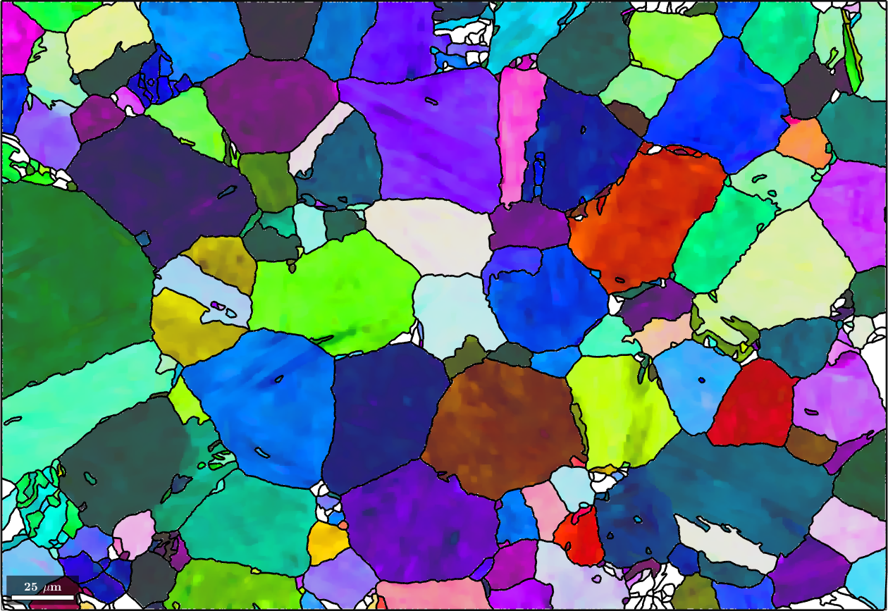
% plot the data and the grain boundaries
plot(ebsd('Iron bcc'),ebsd('Iron bcc').orientations,'figSize','large')
hold on
plot(grains.boundary,'linewidth',2)
hold off

ebsd = EBSD
 
 Phase  Orientations         Mineral         Color  Symmetry  Crystal reference frame
     0   92415 (27%)      notIndexed                                                 
     1  251187 (73%)  Iron bcc (old)  LightSkyBlue       432                         
 
 Properties: bands, bc, bs, error, mad, reliabilityindex
 Scan unit : um
 X x Y x Z : [0 353] x [0 242] x [0 0]
 Normal vector: (0,0,1)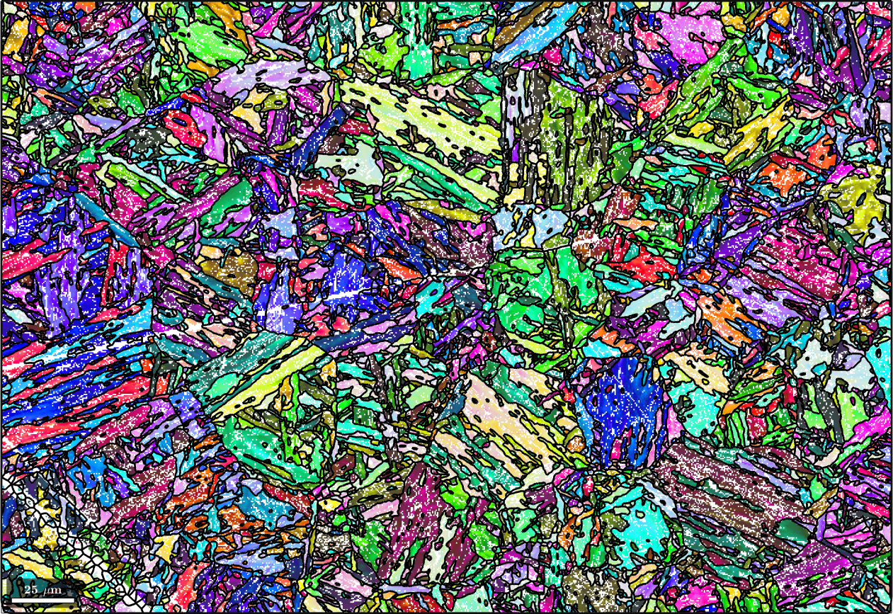

Setting up the parent grain reconstructor

Grain reconstruction is guided in MTEX by a variable of type parentGrainReconstructor. During the reconstruction process this class keeps track about the relationship between the measured child grains and the recovered parent grains.

% set up the job
job = parentGrainReconstructor(ebsd,grains);

The parentGrainReconstructor guesses from the EBSD data what is the parent and what is the child phase. If this guess is not correct it might be specified explicitly by defining an initial guess for the parent to child orientation relationship first and passing it as a third argument to parentGrainReconstructor. Here we define this initial guess separately as the Kurdjumov Sachs orientation relationship

% initial guess for the parent to child orientation relationship
job.p2c = orientation.KurdjumovSachs(job.csParent, job.csChild)
%job.p2c = orientation.NishiyamaWassermann(job.csParent, job.csChild)

job = parentGrainReconstructor
 
 phase   mineral         symmetry  grains  area  reconstructed
 parent  Iron fcc        432       0       0%    0%           
 child   Iron bcc (old)  432       10641   100%               
 
 OR: (111) || (011)   [10-1] || [11-1]
   c2c fit: 2.5°, 3.5°, 4.4°, 5.3° (quintiles)

The output of the variable job tells us the amount of parent and child grains as well as the percentage of already recovered parent grains. Furthermore, it displays how well the current guess of the parent to child orientation relationship fits the child to child misorientations within our data. In our sample data set this fit is described by the 4 quintiles 2.5°, 3.5°, 4.5° and 5.5°.

Optimizing the parent child orientation relationship

It is well known that the phase transformation from austenite to martensite is not described by a fixed orientation relationship. In fact, the actual orientation relationship needs to be determined for each sample individually. Here, we used the iterative method proposed by Tuomo Nyyssönen and implemented in the function calcParent2Child that starts at our initial guess of the orientation relation ship and iterates towards a more optimal orientation relationship.

close all
histogram(job.calcGBFit./degree,'BinMethod','sqrt')
xlabel('disorientation angle')

job.calcParent2Child

ans = parentGrainReconstructor
 
 phase   mineral         symmetry  grains  area  reconstructed
 parent  Iron fcc        432       0       0%    0%           
 child   Iron bcc (old)  432       10641   100%               
 
 OR: (346.1°,9°,58°)
   c2c fit: 1.3°, 1.8°, 2.2°, 2.9° (quintiles)
   closest ideal OR: (111) || (011)   [1-10] || [100] fit: 2.5°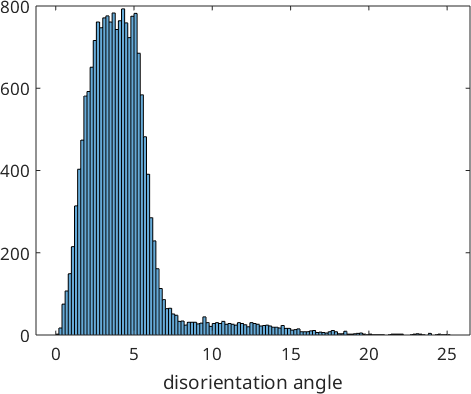

We observe that the optimized parent to child orientation relationship is 2.3° off the initial Kurdjumov Sachs orientation relationship and reduced the first quintil of the misfit with the child to child misorientations to 1.5°. These misfits are stored by the command calcParent2Child in the variable job.fit. In fact, the algorithm assumes that the majority of all boundary misorientations are child to child misorientations and finds the parent to child orientations relationship by minimizing this misfit. The following histogram displays the distribution of the misfit over all grain to grain misorientations.

hold on
histogram(job.calcGBFit./degree,'BinMethod','sqrt')
hold off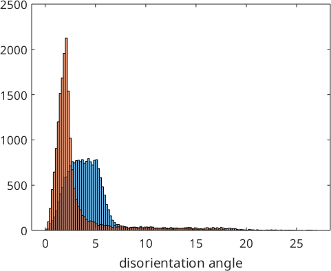

We may explicitly compute the misfit for all child to child boundaries using the command calcGBFit. Beside the list fit it returns also the list of grain pairs for which these fits have been computed. Using the command selectByGrainId we can find the corresponding boundary segments and colorize them according to this misfit. In the code below we go one step further and adjust the transparency as a function of the misfit.

% compute the misfit for all child to child grain neighbors
[fit,c2cPairs] = job.calcGBFit;

% select grain boundary segments by grain ids
[gB,pairId] = job.grains.boundary.selectByGrainId(c2cPairs);

% plot the child phase
plot(ebsd('Iron bcc'),ebsd('Iron bcc').orientations,'figSize','large','faceAlpha',0.5)

% and on top of it the boundaries colorized by the misfit
hold on;
% scale fit between 0 and 1 - required for edgeAlpha
plot(gB, 'edgeAlpha', (fit(pairId) ./ degree - 2.5)./2 ,'linewidth',2);
hold off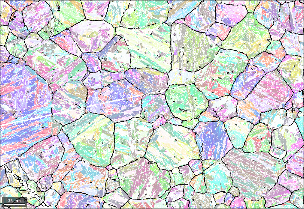

Graph based parent grain reconstruction

Next we set up a graph where each edge describes two neighboring grains and the value of this edge is the probability that these two grains belong to the same parent grain. This graph is computed by the function calcGraph. The probability is computed from the misfit of the misorientation between the two child grains to the theoretical child to child misorientation. More precisely, we model the probability by a cumulative Gaussian distribution with the mean value 'threshold' which describes the misfit at which the probability is exactly 50 percent and the standard deviation 'tolerance'.

job.calcGraph('threshold',2.5*degree,'tolerance',2.5*degree)

ans = parentGrainReconstructor
 
 phase   mineral         symmetry  grains  area  reconstructed
 parent  Iron fcc        432       0       0%    0%           
 child   Iron bcc (old)  432       10641   100%               
 
 OR: (346.1°,9°,58°)
   c2c fit: 1.3°, 1.7°, 2.2°, 3° (quintiles)
   closest ideal OR: (111) || (011)   [1-10] || [100] fit: 2.5°
 
 graph: 10639 grains in 2 clusters + 2 single grain clusters

We may visualize the graph adjusting the edgeAlpha of the boundaries between grains according to the edge value of the graph. This can be accomplished by the command plotGraph

plot(ebsd('Iron bcc'),ebsd('Iron bcc').orientations,'figSize','large','faceAlpha',0.5)
hold on;
job.plotGraph('linewidth',2)
hold off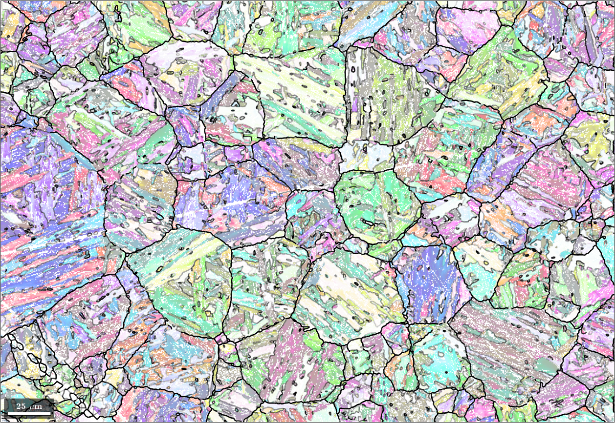

The next step is to cluster the graph into components. This is done by the command clusterGraph which uses by default the Markovian clustering algorithm. The number of clusters can be controlled by the option 'inflationPower'. A smaller inflation power results in fewer but larger clusters.

job.clusterGraph('inflationPower',1.6)

ans = parentGrainReconstructor
 
 phase   mineral         symmetry  grains  area  reconstructed
 parent  Iron fcc        432       0       0%    0%           
 child   Iron bcc (old)  432       10641   100%               
 
 OR: (346.1°,9°,58°)
   c2c fit: 1.3°, 1.8°, 2.2°, 2.9° (quintiles)
   closest ideal OR: (111) || (011)   [1-10] || [100] fit: 2.5°
 
 graph: 10533 grains in 331 clusters + 108 single grain clusters

Finally, we assume a single parent orientation for each cluster and use it to compute a parent orientation for each child grain being part of a cluster. This is done by the command calcParentFromGraph.

% compute parent orientations
job.calcParentFromGraph

% plot them
plot(job.parentGrains,job.parentGrains.meanOrientation)

ans = parentGrainReconstructor
 
 phase   mineral         symmetry  grains  area   reconstructed
 parent  Iron fcc        432       10533   100%   99%          
 child   Iron bcc (old)  432       108     0.14%               
 
 OR: (346.1°,9°,58°)
   p2c fit: 4.3°, 5°, 8.9°, 19° (quintiles)
   c2c fit: 7.2°, 7.2°, 7.2°, 7.2° (quintiles)
   closest ideal OR: (111) || (011)   [1-10] || [100] fit: 2.5°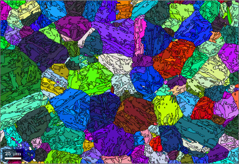

We observe that almost all child grains have been flipped into parent grains. The command calcParentFromGraph has two additional outputs. The misorientation angle between the reconstructed parent orientation of each child grain and the mean parent orientation of the corresponding parent grain is stored in job.grains.fit while job.grains.clusterSize contains the size of each cluster.

figure
plot(job.grains,job.grains.fit./degree)
%plot(job.grains, job.grains.clusterSize < 15)
setColorRange([0,5])
mtexColorbar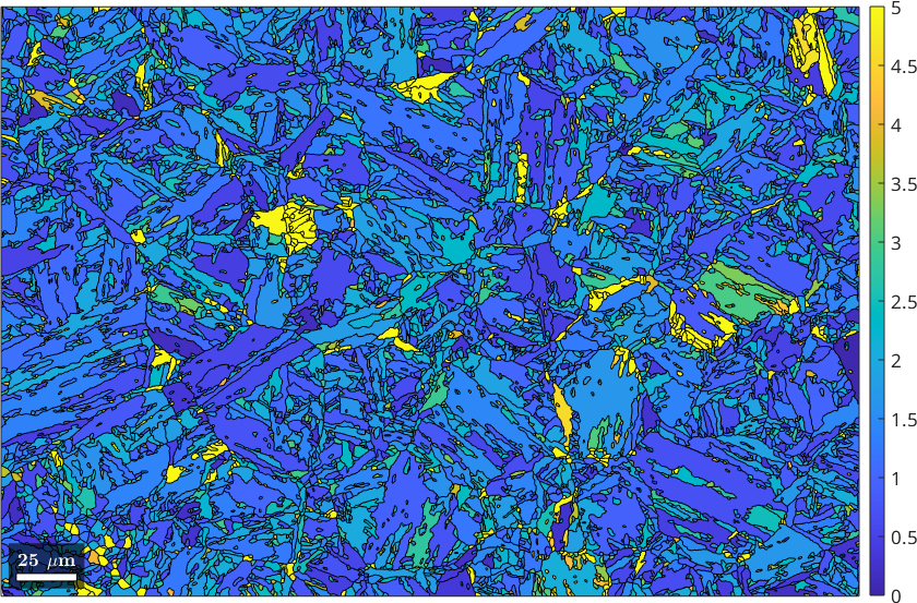

We may use these quantities to undo the parent orientation reconstruction for child grains with a misfit exceeding a certain threshold or belonging to a too small cluster. This can be done by the command job.revert

job.revert(job.grains.fit > 5*degree | job.grains.clusterSize < 15)

plot(job.parentGrains,job.parentGrains.meanOrientation)

ans = parentGrainReconstructor
 
 phase   mineral         symmetry  grains  area  reconstructed
 parent  Iron fcc        432       8990    92%   84%          
 child   Iron bcc (old)  432       1651    8%                 
 
 OR: (346.1°,9°,58°)
   p2c fit: 4°, 8.3°, 13°, 20° (quintiles)
   c2c fit: 1.2°, 1.7°, 2.1°, 2.9° (quintiles)
   closest ideal OR: (111) || (011)   [1-10] || [100] fit: 2.5°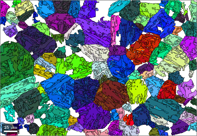

When used without any input argument job.revert will undo all reconstructed parent grain. This is helpful when experimenting with different parameters.

In order to fill the holes corresponding to the remaining child grains we inspect their misorientations to neighboring already reconstructed parent grains. Each of these misorientations votes for a certain parent orientation. We choose the parent orientation that gets the most votes. The corresponding commands job.calcGBVotes and job.calcParentFromVote can be adjusted by many options.

for k = 1:3 % do this three times

  % compute votes
  job.calcGBVotes('p2c','threshold', k * 2.5*degree);

  % compute parent orientations from votes
  job.calcParentFromVote
end

% plot the result
plot(job.parentGrains,job.parentGrains.meanOrientation)

ans = parentGrainReconstructor
 
 phase   mineral         symmetry  grains  area  reconstructed
 parent  Iron fcc        432       9438    95%   89%          
 child   Iron bcc (old)  432       1203    4.8%               
 
 OR: (346.1°,9°,58°)
   p2c fit: 5.2°, 10°, 14°, 21° (quintiles)
   c2c fit: 1.2°, 1.7°, 2.2°, 3.2° (quintiles)
   closest ideal OR: (111) || (011)   [1-10] || [100] fit: 2.5°
 
 votes: 5 x 1
   probabilities: 0%, 0%, 0%, 0% (quintiles)
 
 
ans = parentGrainReconstructor
 
 phase   mineral         symmetry  grains  area  reconstructed
 parent  Iron fcc        432       9975    97%   94%          
 child   Iron bcc (old)  432       666     2.7%               
 
 OR: (346.1°,9°,58°)
   p2c fit: 11°, 13°, 17°, 23° (quintiles)
   c2c fit: 1.2°, 1.7°, 2.2°, 3.4° (quintiles)
   closest ideal OR: (111) || (011)   [1-10] || [100] fit: 2.5°
 
 votes: 5 x 1
   probabilities: 0%, 0%, 0%, 0% (quintiles)
 
 
ans = parentGrainReconstructor
 
 phase   mineral         symmetry  grains  area  reconstructed
 parent  Iron fcc        432       10305   99%   97%          
 child   Iron bcc (old)  432       336     1.2%               
 
 OR: (346.1°,9°,58°)
   p2c fit: 15°, 19°, 22°, 26° (quintiles)
   c2c fit: 1.3°, 1.8°, 2.4°, 3.7° (quintiles)
   closest ideal OR: (111) || (011)   [1-10] || [100] fit: 2.5°
 
 votes: 5 x 1
   probabilities: 0%, 0%, 0%, 0% (quintiles)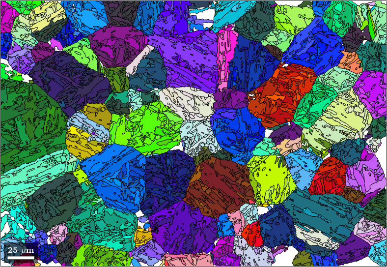

Merge similar grains and inclusions

We observe that we have many neighboring parent grains with similar orientations. These can be merged into big parent grains using the command mergeSimilar

% merge grains with similar orientation
job.mergeSimilar('threshold',7.5*degree);

% plot the result
plot(job.parentGrains,job.parentGrains.meanOrientation)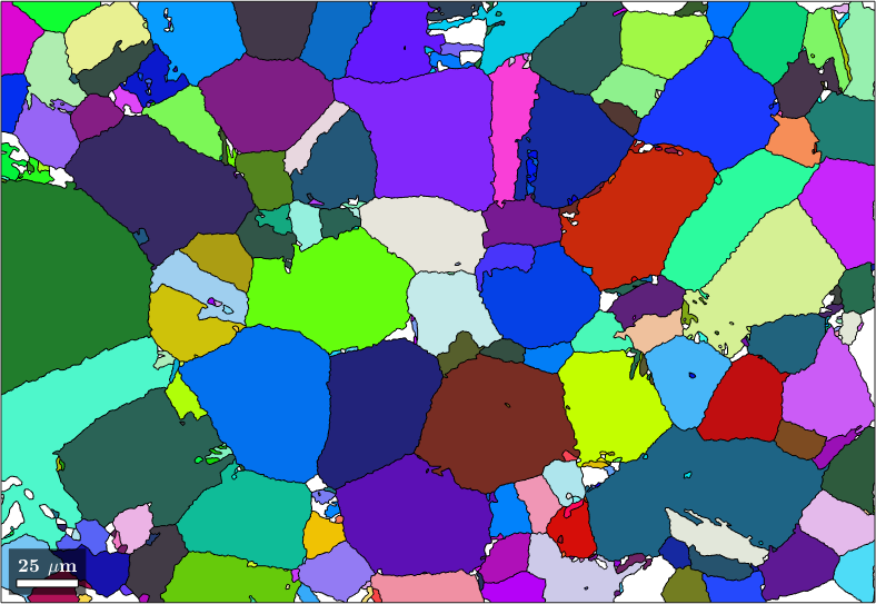

We may be still a bit unsatisfied with the result as the large parent grains contain many poorly indexed inclusions where we failed to assign to a parent orientation. We may use the command mergeInclusions to merge all inclusions with fever pixels then a certain threshold into the surrounding parent grains.

job.mergeInclusions('maxSize',50);

% plot the result
plot(job.parentGrains,job.parentGrains.meanOrientation)

Compute Child Variants

Knowing the parent grain orientations we may compute the variants and packets of each child grain using the command calcVariants. The values are stored with the properties job.transformedGrains.variantId and job.transformedGrains.packetId. The packetId is defined as the closest {111} plane in austenite to the (011) plane in martensite.

job.calcVariants

% associate to each packet id a color and plot
color = ind2color(job.transformedGrains.packetId);
plot(job.transformedGrains,color,'faceAlpha',0.5)

hold on
parentGrains = smooth(job.parentGrains,10);
plot(parentGrains.boundary,'linewidth',3)

% outline a specific parent grain
grainSelected = parentGrains(parentGrains.findByLocation([100,80]));

hold on
plot(grainSelected.boundary,'linewidth',3,'lineColor','w')
hold off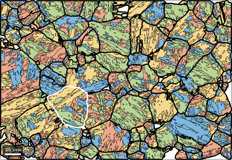

We can also directly identify the child grains belonging to the selected parent grains. Remember that the initial grains are stored in job.grainsPrior and that the vector job.mergeId stores for every initial grain the id of the corresponding parent grain. Combining these two information we do

% identify childs of the selected parent grain
childGrains = job.grainsPrior(job.mergeId == grainSelected.id);

% plot these childs
plot(childGrains,childGrains.meanOrientation)

% and top the parent grain boundary
hold on
plot(grainSelected.boundary,'linewidth',2)
hold off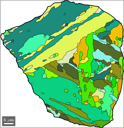

In order to check our parent grain reconstruction we chose the single parent grain outlined in the above map and plot all child variants of its reconstructed parent orientation together with the actually measured child orientations inside the parent grain. In order to compute the variantId and packetId we use the command calcVariantId.

% the measured child orientations that belong to parent grain 279
childOri = job.ebsdPrior(childGrains).orientations;

% the orientation of parent grain 279
parentOri = grainSelected.meanOrientation;

% lets compute the variant and packeIds
[variantId, packetId] = calcVariantId(parentOri,childOri,job.p2c);

% colorize child orientations by packetId
color = ind2color(packetId);
plotPDF(childOri,color, Miller(0,0,1,childOri.CS),'MarkerSize',2,'all')

% the positions of the parent (001) directions
hold on
plot(parentOri.symmetrise * Miller(0,0,1,parentOri.CS),'markerSize',10,...
  'marker','s','markerFaceColor','w','MarkerEdgeColor','k','linewidth',2)

% the theoretical child variants
childVariants = variants(job.p2c, parentOri);
plotPDF(childVariants, 'markerFaceColor','none','linewidth',1.5,'markerEdgeColor','k')
hold off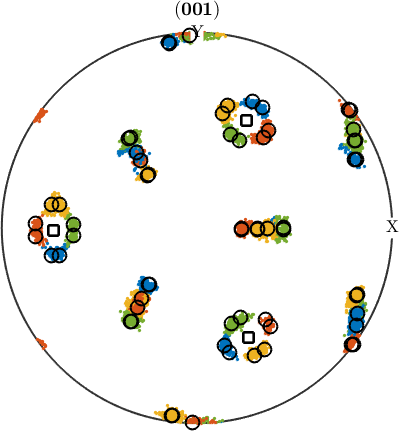

Parent EBSD reconstruction

So far our analysis was at the grain level. However, once parent grain orientations have been computed we may also use them to compute parent orientations of each pixel in our original EBSD map. This is done by the command calcParentEBSD

parentEBSD = job.calcParentEBSD;

% plot the result
plot(parentEBSD('Iron fcc'),parentEBSD('Iron fcc').orientations,'figSize','large')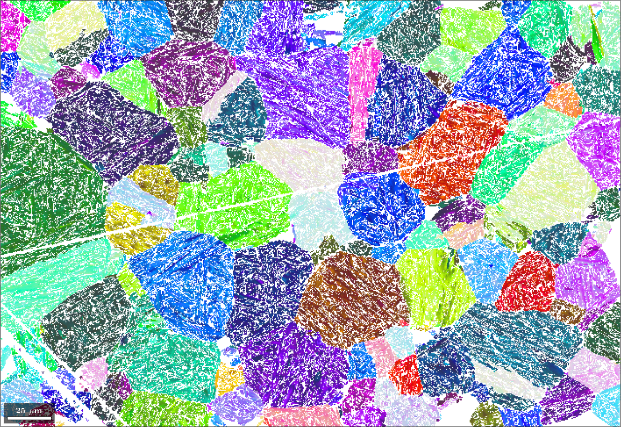

We obtain even a measure parentEBSD.fit for the correspondence between the parent orientation reconstructed from the single pixel and the parent orientation of the grain. Lets visualize this fit

% the fit between ebsd child orientation and the reconstructed parent grain
% orientation
plot(parentEBSD, parentEBSD.fit ./ degree,'figSize','large')
mtexColorbar
setColorRange([0,5])
mtexColorMap('LaboTeX')

hold on
plot(job.grains.boundary,'lineWidth',2)
hold off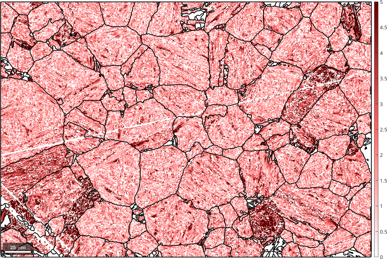

Denoise the parent map

Finally, we may apply filtering to the parent map to fill non indexed or not reconstructed pixels. To this end we first run grain reconstruction on the parent map

[parentGrains, parentEBSD.grainId] = calcGrains(parentEBSD('indexed'),'angle',3*degree);

% remove very small grains
parentEBSD(parentGrains(parentGrains.grainSize<10)) = [];

% redo grain reconstruction
[parentGrains, parentEBSD.grainId] = calcGrains(parentEBSD('indexed'),'angle',3*degree);
parentGrains = smooth(parentGrains,10);

plot(ebsd('indexed'),ebsd('indexed').orientations,'figSize','large')

hold on
plot(parentGrains.boundary,'lineWidth',2)
hold off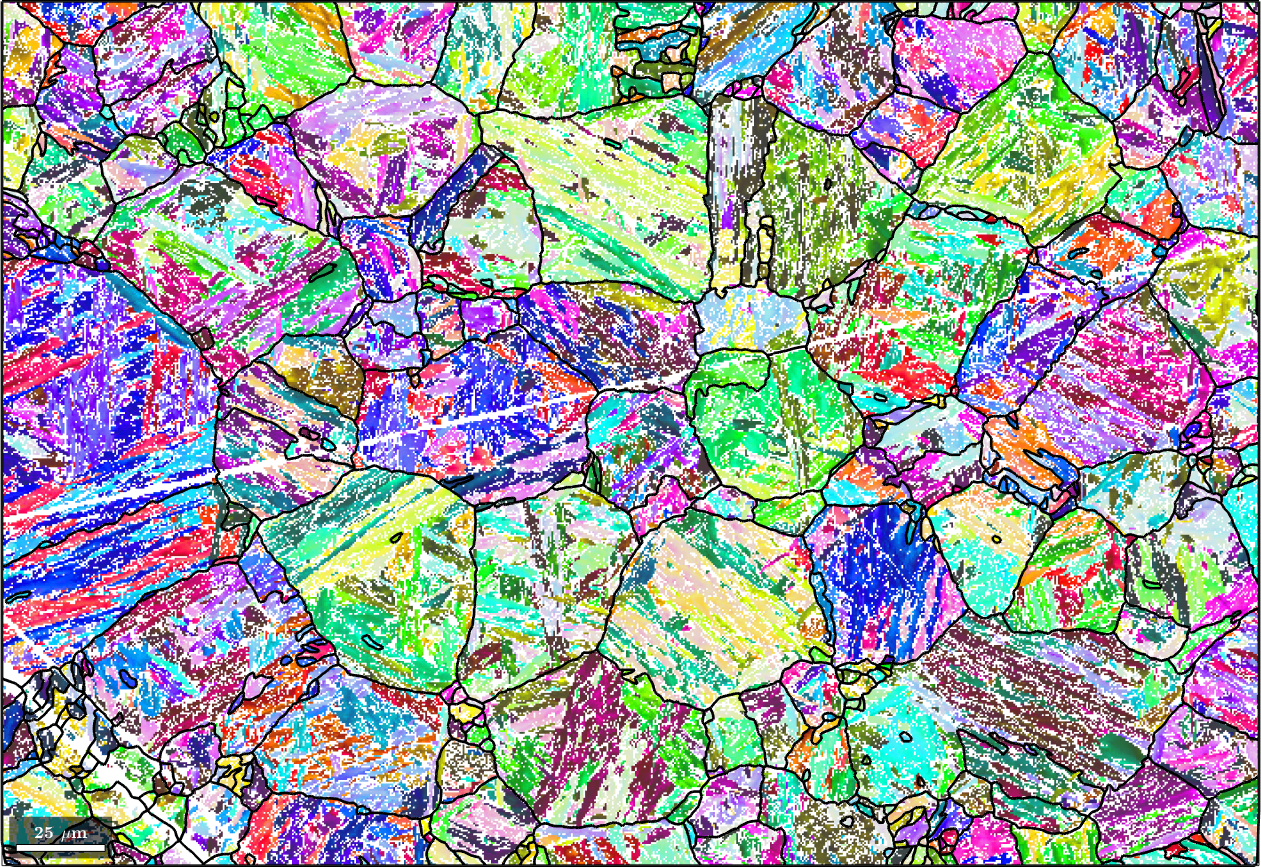

and then use the command smooth to fill the holes in the reconstructed parent map

% fill the holes
F = halfQuadraticFilter;
parentEBSD = smooth(parentEBSD('indexed'),F,'fill',parentGrains);

% plot the parent map
plot(parentEBSD('Iron fcc'),parentEBSD('Iron fcc').orientations,'figSize','large')

% with grain boundaries
hold on
plot(parentGrains.boundary,'lineWidth',2)
hold off