Export Pole Figure Data

export writes the sampled directions and intensities of a PoleFigure to plain ASCII tables. This page exports measured data, reads it back, and then exports pole figures recalculated from an orientation distribution function (ODF).

The tables are easy to exchange, but they are not a self-describing file format. Keep the crystal and specimen frames, symmetries, angular unit, Miller indices, and superposition coefficients with the files. Importing these quantities is introduced in Import Pole Figure Data. The meaning of a pole figure is explained in Pole Figures.

Start with measured pole figures

The Dubna quartz data set contains seven pole-figure entries. Its specimen frame is drawn with Y pointing up and X pointing right.

plottingConvention.default('y↑→x');
mtexdata dubna silent

pf

pf = PoleFigure (y↑→x)
  crystal symmetry : Quartz (321, X||a*, Y||b, Z||c)
 
  h = (022̅1), r = 72 × 19 points
  h = (101̅0), r = 72 × 19 points
  h = (101̅1)(011̅1), r = 72 × 19 points
  h = (101̅2), r = 72 × 19 points
  h = (112̅0), r = 72 × 19 points
  h = (112̅1), r = 72 × 19 points
  h = (112̅2), r = 72 × 19 points

The summary lists one row per entry. An entry may represent one crystal direction or a superposition of directions whose diffraction peaks could not be resolved. The third Dubna entry is such a superposition, so seven entries do not necessarily mean seven individual reflections.

Write one file per entry

Different pole figures may be measured on different specimen grids. export therefore writes each entry to a separate file instead of assuming one common list of specimen directions. The file name combines the base name below with the entry's Miller indices.

% write into the temporary folder
fname = fullfile(tempdir,'dubna');
export(pf,fname,'degree')

Inspect the files

List the generated files, then show the beginning of the first table.

d = dir([fname,'_*.txt']);
fprintf('Exported %d files:\n',numel(d))
disp({d.name}')

firstFile = fullfile(d(1).folder,d(1).name);
preview = readmatrix(firstFile);
disp('Rows from three successive polar rings: angle, azimuth, intensity')
disp(preview([1,73,145],:))

Exported 7 files:
    {'dubna_(022̅1).txt'      }
    {'dubna_(101̅0).txt'      }
    {'dubna_(101̅1)(011̅1).txt'}
    {'dubna_(101̅2).txt'      }
    {'dubna_(112̅0).txt'      }
    {'dubna_(112̅1).txt'      }
    {'dubna_(112̅2).txt'      }
Rows from three successive polar rings: angle, azimuth, intensity
         0         0         0
    5.0000  272.5000         0
   10.0000  275.0200         0

Every row has three columns: the polar angle of the specimen direction, its azimuth angle, and the measured diffraction intensity. The 'degree' option writes both angles in degrees; without it, export writes radians.

The files contain numbers only. In particular, they do not contain column labels, angular units, crystal or specimen symmetry, crystal-frame alignment, specimen-frame identity, or superposition coefficients. The Miller indices appear in the file name, but a naming convention is not a substitute for metadata. When sharing the tables, include a script or README that records these choices and explains how specimen X, Y, and Z correspond to the physical sample.

Read the data back

The three columns are exactly those understood by loadPoleFigure_generic. To reconstruct the object, PoleFigure.load also needs the Miller indices, crystal and specimen symmetries, and superposition coefficients that were not stored in the tables.

% reconstruct the file names from the Miller indices
fnames = cellfun(@(h) [fname,'_',char(h),'.txt'],pf.allH,...
  'UniformOutput',false);

pf2 = PoleFigure.load(fnames,pf.allH,pf.CS,pf.SS,...
  'superposition',pf.c,...
  'ColumnNames',{'polar angle','azimuth angle','intensity'},'degree')

pf2 = PoleFigure (y↑→x)
  crystal symmetry : Quartz (321, X||a*, Y||b, Z||c)
 
  h = (022̅1), r = 1368 × 1 points
  h = (101̅0), r = 1368 × 1 points
  h = (101̅1)(011̅1), r = 1368 × 1 points
  h = (101̅2), r = 1368 × 1 points
  h = (112̅0), r = 1368 × 1 points
  h = (112̅1), r = 1368 × 1 points
  h = (112̅2), r = 1368 × 1 points

Check the round trip

ASCII output has finite decimal precision. Report the largest intensity change introduced by writing and reading the tables.

roundTripError = max(abs(pf.intensities(:) - pf2.intensities(:)));
fprintf('Maximum absolute intensity change: %.3g\n',roundTripError)

Maximum absolute intensity change: 0

For these files the printed maximum intensity change is zero. The specimen directions and intensities therefore survive to the printed precision. The regular \(72 \times 19 = 1368\) grid structure does not: each reloaded entry stores the same 1368 specimen directions as a plain list. This makes no difference to MTEX computations that use those directions, but software that needs the original row-and-column layout must reconstruct it from separately recorded acquisition information.

Plot the reloaded data

plot(pf2,'figSize','small')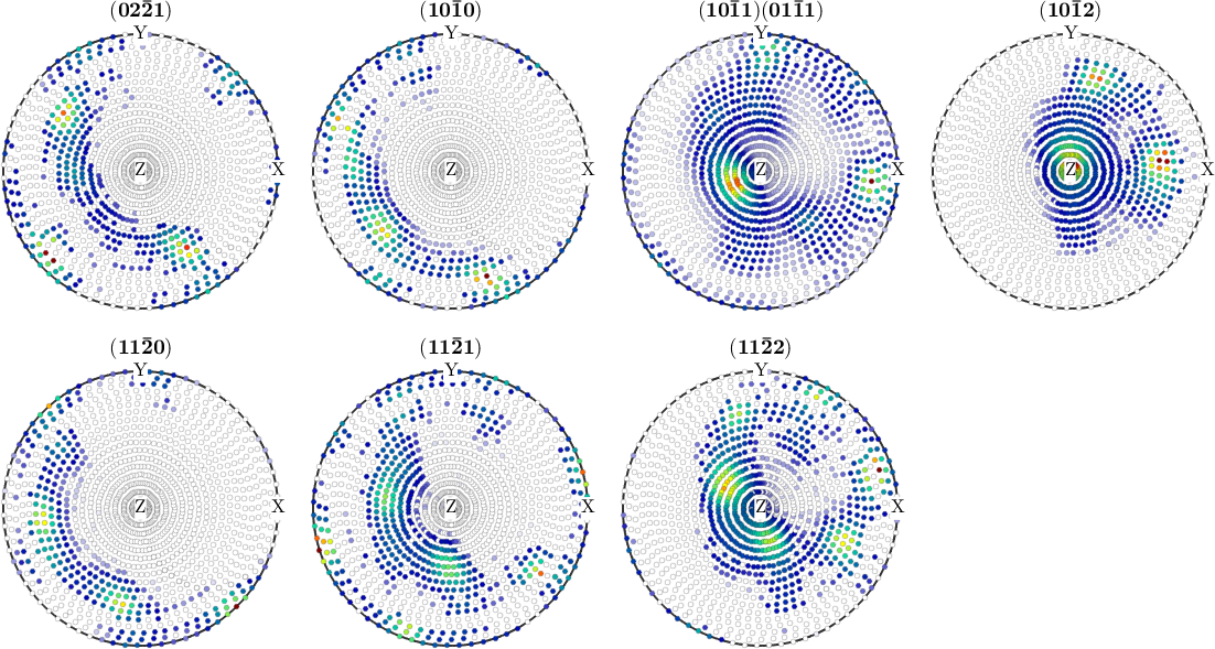

The seven panels retain the measured bands, maxima, and angular coverage. A plot is a useful check for swapped angle columns, wrong angular units, or a mismatched specimen frame. It cannot reveal missing symmetry or superposition metadata when the numeric values themselves are unchanged.

Export recalculated pole figures

The same command exports pole figures computed from an ODF with calcPoleFigure. This is useful when another program needs directional pole-density samples rather than the ODF itself.

odf = calcODF(pf,'silent');

pfSim = calcPoleFigure(odf,pf.allH,pf.allR,...
  'superposition',pf.c);

Superposition coefficients must be passed explicitly. The third Dubna pole figure combines \((10\bar{1}1)\) and \((01\bar{1}1)\) with the weights in pf.c{3}. Without them, calcPoleFigure would average the two contributions with equal default weights and calculate different intensities.

recalculatedName = fullfile(tempdir,'dubnaRecalculated');
export(pfSim,recalculatedName,'degree')

Clean up

Remove the temporary files after the inspection and round-trip check.

delete([fname,'_*.txt'])
delete([recalculatedName,'_*.txt'])

Choose the quantity to exchange

Export pole figures when the receiving program needs intensities or pole densities sampled over specimen directions. If the starting quantity is an ODF, exporting only selected pole figures discards information: a finite set of pole figures does not determine an ODF uniquely. Use ODF Export when the receiving program can accept an ODF or a discrete representation of it.

Further reading

Next

ODF Analysis develops the continuous quantity usually reconstructed from measured pole figures. Continue to ODF Export to compare its component, grid, and discrete-orientation formats.