ODF Export

Exporting an orientation distribution function (ODF) means choosing what the receiving program needs. MTEX supports four common representations:

The last two are finite approximations to the continuous ODF introduced in ODF Theory. Record the Euler-angle convention, angle units, grid resolution or number of orientations, crystal symmetry and specimen symmetry whenever the result must be reproducible.

Define a Model ODF

The examples use one mixture of uniform, fibre and unimodal components. Keeping the ODF fixed makes the differences between the file formats visible.

cs = crystalSymmetry('cubic');
mod1 = orientation.byAxisAngle(xvector,45*degree,cs);
mod2 = orientation.byAxisAngle(yvector,65*degree,cs);
model_odf = 0.5*uniformODF(cs) + ...
  0.05*fibreODF(Miller(1,0,0,cs),xvector,'halfwidth',10*degree) + ...
  0.05*fibreODF(Miller(0,1,0,cs),yvector,'halfwidth',10*degree) + ...
  0.05*fibreODF(Miller(0,0,1,cs),zvector,'halfwidth',10*degree) + ...
  0.05*unimodalODF(mod1,'halfwidth',15*degree) + ...
  0.3*unimodalODF(mod2,'halfwidth',25*degree);
plot(model_odf,'sections',6,'silent')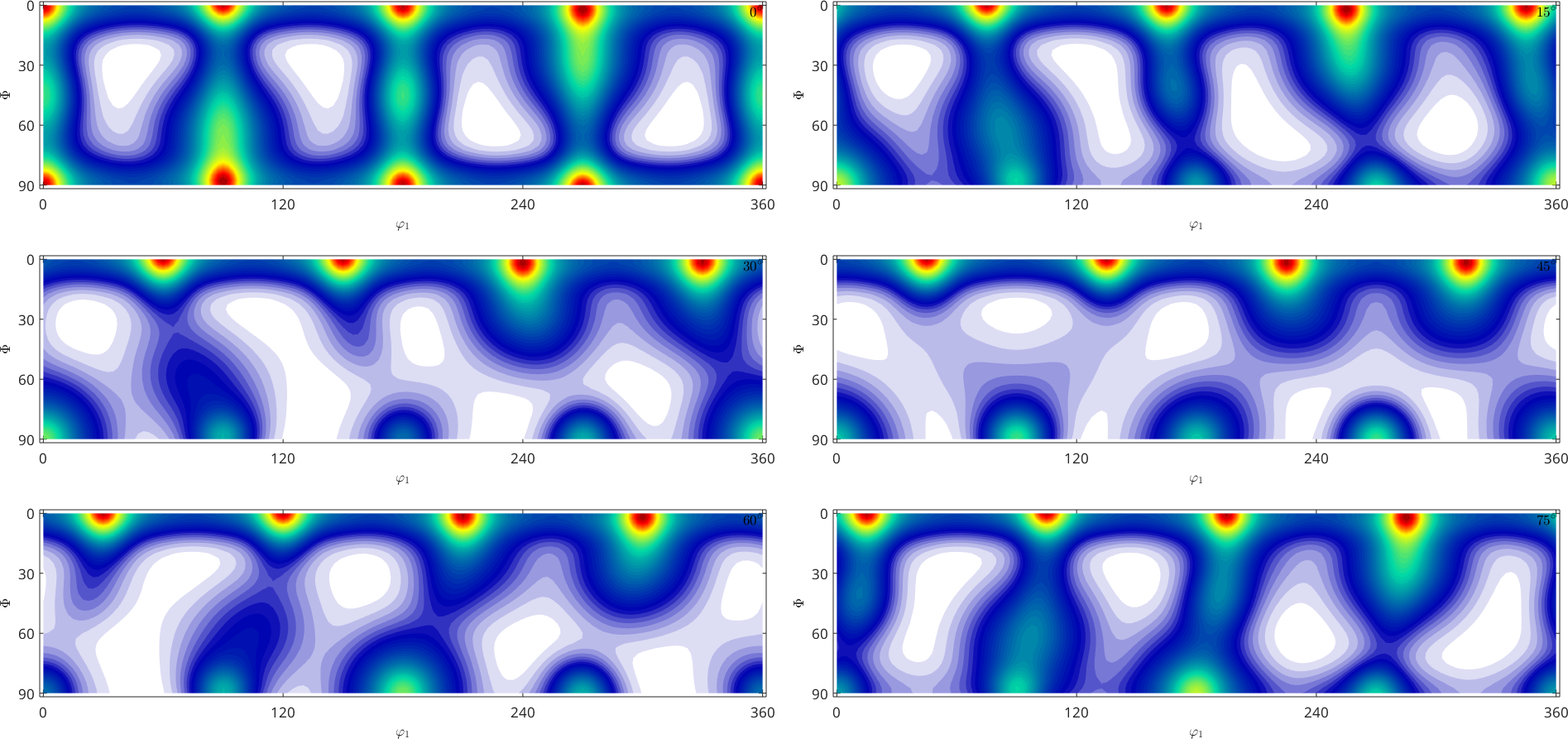

The six sections show a smooth density with localized maxima and fibre ridges on a uniform background. The grid and VPSC exports below replace this continuous function by finitely many rows.

Save a MATLAB Object

Use MATLAB's save when the next step also runs in MATLAB with MTEX. Unlike a table export, this stores model_odf itself. Pass the variable name to save as text.

matName = fullfile(tempdir,'odf.mat');
save(matName,'model_odf')

Loading the file returns the stored ODF object rather than reconstructing one from sampled values. The assertion makes that round trip executable.

saved = load(matName,'model_odf');
assert(isa(saved.model_odf,'SO3FunComposition') && ...
  isequal(eval(saved.model_odf,[mod1,mod2]),eval(model_odf,[mod1,mod2])))

Export Values on a Generic Grid

By default, export writes four columns. The first three are Bunge Euler angles on a regular \(5^\circ\) grid, in degrees, and the fourth is the ODF value at that orientation. These values are density values in multiples of a uniform distribution, not volume fractions.

Sampling does not preserve the internal ODF representation. A grid that is too coarse can miss a narrow component, so choose the resolution from the smallest feature that the receiving calculation must resolve. Here we request \(10^\circ\) to keep the example file compact.

genericName = fullfile(tempdir,'odf-generic.txt');
export(model_odf,genericName,'Bunge','resolution',10*degree)

The header records the symmetries and names the four columns. The first data rows then contain angles and the sampled ODF value.

disp('Beginning of the generic grid file:')
fid = fopen(genericName);
for k = 1:6, disp(fgetl(fid)); end
fclose(fid);

Beginning of the generic grid file:
% MTEX ODF
% crystal symmetry: "m-3m"
% specimen symmetry: "1"
% phi1    Phi     phi2    value
0.00000 0.00000 0.00000 3.46659
10.00000 0.00000 0.00000 2.63068

Pass a Grid Directly

Other Euler-angle conventions and resolutions are available as options to export. For complete control, construct an orientation grid and pass it directly. This example uses an equispaced grid with a nominal resolution of \(10^\circ\).

S3G = equispacedSO3Grid(cs,'resolution',10*degree);
gridName = fullfile(tempdir,'odf-equispaced.txt');
export(model_odf,gridName,S3G,'Bunge','generic')

Export an MTEX Component Description

The 'mtex' interface writes a human-readable description of the ODF components. It records the components themselves instead of replacing them by grid samples, and it is not a general interchange format.

The current source tree has no matching reader: SO3Fun.load offers loaders for generic and VPSC ODF files only, so this format is write-only. Use .mat when an exact round trip matters. Not every representation is supported either, and the exporter records that harmonic components cannot be written in this format.

mtexName = fullfile(tempdir,'odf.mtex');
export(model_odf,mtexName,'Bunge','interface','mtex')

The beginning of the file identifies the symmetries and the uniform component. Later blocks describe the fibre and radial components.

disp('Beginning of the MTEX component file:')
fid = fopen(mtexName);
for k = 1:8, disp(fgetl(fid)); end
fclose(fid);

Beginning of the MTEX component file:
% MTEX ODF
% crystal symmetry: "m-3m"
% specimen symmetry: "1"
%
%% uniform component
% weight: 0.50000
%
%% fibre component

Export a Synthetic Polycrystal for VPSC

The VPSC code and other crystal plasticity programs operate on discrete crystal orientations rather than directly on an ODF. The 'VPSC' interface therefore draws orientations from the ODF and writes their Bunge Euler angles and volume fractions.

vpscName = fullfile(tempdir,'odf-vpsc.txt');
export(model_odf,vpscName,'VPSC','points',5000)

A VPSC block has four header lines. Its fourth line gives the Euler-angle convention and orientation count: B means Bunge. Each following row contains three Euler angles in degrees and one volume fraction.

disp('Beginning of the VPSC file:')
fid = fopen(vpscName);
for k = 1:6, fprintf('%s\n',fgetl(fid)); end
fclose(fid);

Beginning of the VPSC file:
texture exported by MTEX


B 5000
 107.10  150.76  172.21   0.0002000
 259.28   82.73   11.32   0.0002000

The 'points' option controls the number of orientations and defaults to 10000. More orientations usually represent the continuous density more finely, but they also make the receiving calculation larger. A VPSC file carries no crystal symmetry, so pass that information separately when it is read. Import from VPSC shows the return path.

Clean Up

All examples wrote to MATLAB's temporary directory. Remove every file now that the previews and round-trip check are complete.

delete(matName)
delete(genericName)
delete(gridName)
delete(mtexName)
delete(vpscName)

Choosing a Format

Use .mat while continuing an analysis in MATLAB and MTEX. Use MTEX ASCII when a readable description of supported components is useful. Use a generic grid when the receiving program expects function values, and use VPSC when it expects a synthetic polycrystal.

Grid spacing and sample size are accuracy parameters, not merely file-format options. Random Sampling explains why a random statistical sample and an optimized numerical representation are not interchangeable. ODF Import explains how MTEX interprets tabulated values and weights when files are read back. Orientation Export is the corresponding page when the starting data are already individual orientations rather than an ODF.

References

- H.-J. Bunge, Texture Analysis in Materials Science: Mathematical Methods, Butterworths, 1982. This is the standard reference for ODFs and the Bunge Euler-angle convention.
- R. A. Lebensohn and C. N. Tomé, A self-consistent anisotropic approach for the simulation of plastic deformation and texture development of polycrystals, Acta Metallurgica et Materialia 41 (1993), 2611--2624. This paper introduces the VPSC formulation used by the discrete-orientation export.
Citing this page.
This page is part of the documentation of
MTEX, a free and open
source MATLAB toolbox for analyzing and modeling crystallographic textures.
It was written by The MTEX Developers and is published at
https://mtex-toolbox.github.io/ODFExport.html.
If you use MTEX, or reuse text or figures from this page, in your research,
please cite
F. Bachmann, R. Hielscher, H. Schaeben: Texture Analysis with MTEX - Free and Open Source Software Toolbox, Solid State Phenomena 160 (2010), 63-68. 10.4028/www.scientific.net/SSP.160.63
BibTeX
@article{bachmann2010mtex,
author  = {F. Bachmann and R. Hielscher and H. Schaeben},
title   = {Texture Analysis with MTEX - Free and Open Source Software Toolbox},
journal = {Solid State Phenomena},
volume  = {160},
pages   = {63-68},
year    = {2010},
doi     = {10.4028/www.scientific.net/SSP.160.63},
url     = {https://doi.org/10.4028/www.scientific.net/SSP.160.63}
}
Other papers describing specific MTEX methods are listed under Publications — please cite the one that best fits your application. The MTEX source code is licensed under the GNU General Public License v2.0; the text and figures of this documentation are licensed under CC BY 4.0, which permits reuse — including by automated systems — provided The MTEX Developers and this page are credited.