In the section density estimation we have seen that the correct choice of the kernel halfwidth is essential for creating a good match between the true density function and the reconstructed density function. If the halfwidth is set too small the reconstructed density function is usually oscillating and the individual sampling points are visible as sharp peaks. If the halfwidth is too large the resulting density function is usually too smooth and does not reproduce the features of the original density function.
Finding an optimal kernel halfwidth is a hard problem as the optimal kernel halfwidth depends not only on the number of sampling points but also on the smoothness of the true but unknown density function. MTEX offers several options set by flags during the kernel calculation operation. A very conservative choice for the kernel halfwidth that takes into account only the number of sampling points is implemented in MTEX with the flag 'magicRule'. The flag 'RuleOfThumb' considers both the number of sampling points and the variance of the sampling points as an estimate of the smoothness of the true density function. The most advanced (and default) method for estimating the optimal kernel halfwidth is Kullback Leibler cross validation. This method tests different kernel half-widths on a subset of the random sample and selects the halfwidth which best reproduces the omitted points of the random sample.
In order to demonstrate this functionality let's start with the following orientation density function
% cubic crystal symmetry
cs = crystalSymmetry('321');

% build a density function by combining a uniform texture with two
% predefined texture components
odf = 0.25*uniformODF(cs) + ...
  0.25 * unimodalODF(orientation.byEuler([35,45,0]*degree,cs)) + ...
  0.5 * fibreODF(Miller(7,-1,10,cs),vector3d(7,-5,11),'halfwidth',10*degree);

% plot the density function as six sigma sections
plot(odf,'sections',6,'silent','sigma')
mtexColorbar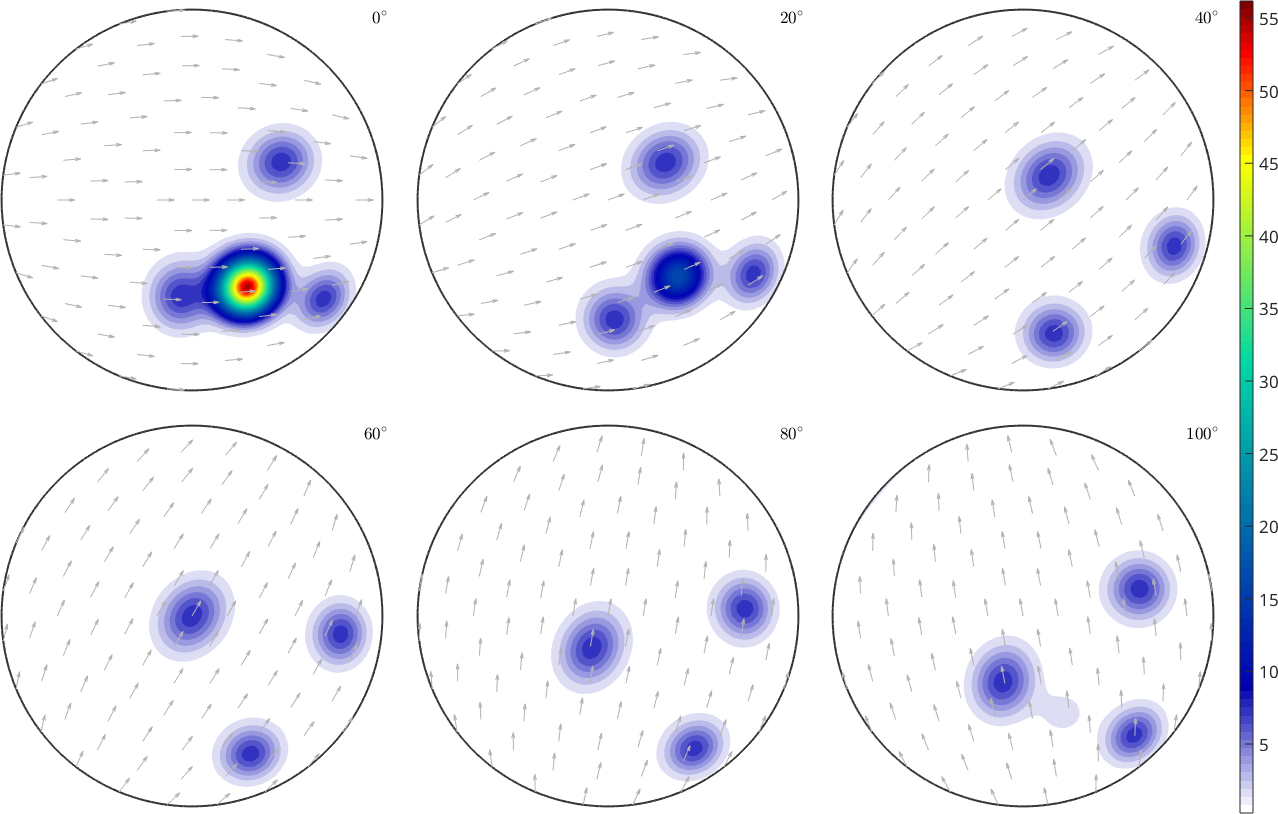
and compute \(10000\) random orientations representing this density function using the command discreteSample
ori = odf.discreteSample(10000)ori = orientation (321 → y↑→x)
size: 10000 x 1Next we estimate the optimal kernel function using the command calcKernel with the default settings.
psi = calcKernel(ori)psi = SO3DeLaValleePoussinKernel
bandwidth: 43
halfwidth: 5.7°This kernel can now be used to reconstruct the original ODF from the sampled points using the command density estimation
odf_rec = calcDensity(ori,'kernel',psi)

% plot the reconstructed ODF and compare it to the plot of the original function.  The results are similar but not identical.
figure;plot(odf_rec,'sections',6,'silent','sigma')
mtexColorbar
odf_rec = SO3FunHarmonic (321 → y↑→x)
bandwidth: 43
weight: 1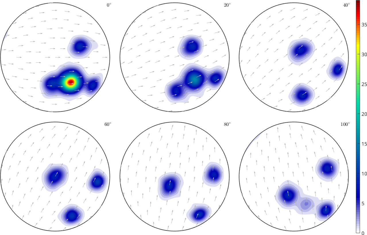
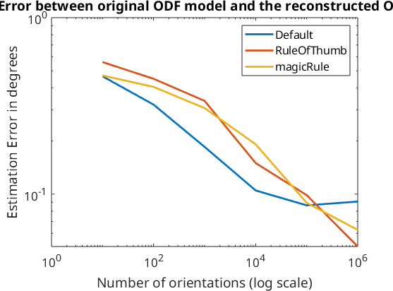
Exploration of the relationship between estimation error and number of single orientations
In this section we want to compare the different methods for estimating the optimal kernel halfwidth. To this end we simulate 10, 100, ..., 1000000 single orientations from the model ODF odf, compute optimal kernels according to the 'magicRule', the 'RuleOfThumb' and Kullback Leibler cross validation and then compute the fit between the reconstructed odf_rec and the original odf.
% define a variable to hold the calculated error values
e = [];
for i = 1:6

  % calculate a sample of orientations from the model ODF
  ori = discreteSample(odf,10^i,'silent');

  % calculate the kernel using the function defaults, reconstruct the odf, and calculate error between this and the original ODF
  psi1 = calcKernel(ori,'SamplingSize',10000,'silent');
  odf_rec = calcDensity(ori,'kernel',psi1,'silent');
  e(i,1) = calcError(odf_rec,odf,'resolution',2.5*degree);

  % calculate the kernel using the RuleOfThumb, reconstruct the odf, and calculate error between this and the original ODF
  psi2 = calcKernel(ori,'method','RuleOfThumb','silent');
  odf_rec = calcDensity(ori,'kernel',psi2,'silent');
  e(i,2) = calcError(odf_rec,odf,'resolution',2.5*degree);

  % calculate the kernel using the magicRule, reconstruct the odf, and calculate error between this and the original ODF
  psi3 = calcKernel(ori,'method','magicRule','silent');
  odf_rec = calcDensity(ori,'kernel',psi3,'silent');
  e(i,3) = calcError(odf_rec,odf,'resolution',2.5*degree);

  % generate text showing the kernel size calculated with each method in each loop
  disp(['RuleOfThumb: ' int2str(psi2.halfwidth/degree) mtexdegchar ...
    ' KLCV: ' int2str(psi1.halfwidth/degree) mtexdegchar ...
    ' magicRule: ' int2str(psi3.halfwidth/degree) mtexdegchar ...
    ]);

end

% Plot the error to the number of single orientations sampled from the original ODF.
close all;
loglog(10.^(1:length(e)),e,'LineWidth',2)
legend('Default','RuleOfThumb','magicRule')
xlabel('Number of orientations (log scale)')
ylabel('Estimation Error in degrees')
title('Error between original ODF model and the reconstructed ODF','FontWeight','bold')
RuleOfThumb: 76° KLCV: 24° magicRule: 31°
RuleOfThumb: 36° KLCV: 15° magicRule: 22°
RuleOfThumb: 18° KLCV: 8° magicRule: 16°
RuleOfThumb: 10° KLCV: 6° magicRule: 11°
RuleOfThumb: 8° KLCV: 5° magicRule: 8°
RuleOfThumb: 7° KLCV: 4° magicRule: 6°