Triple Point Based Parent Phase Reconstruction

Triple Point Based Parent Phase Reconstruction edit page

In this section we discuss triple point based parent grain reconstruction at the example of a titanium alloy. Lets start by importing a sample data set

mtexdata alphaBetaTitanium

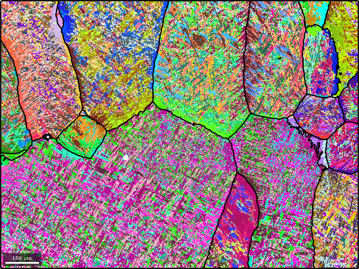
% and plot the alpha phase as an inverse pole figure map
plot(ebsd('Ti (alpha)'),ebsd('Ti (alpha)').orientations,'figSize','large')

ebsd = EBSD
 
 Phase  Orientations     Mineral         Color  Symmetry  Crystal reference frame
     0  10449 (5.3%)  notIndexed                                                 
     1   437 (0.22%)   Ti (BETA)  LightSkyBlue       432                         
     2  185722 (94%)  Ti (alpha)  DarkSeaGreen       622       X||a*, Y||b, Z||c*
 
 Properties: bands, bc, bs, error, mad, reliabilityindex
 Scan unit : um
 X x Y x Z : [0 1568] x [-1175 0] x [0 0]
 Normal vector: (0,0,-1)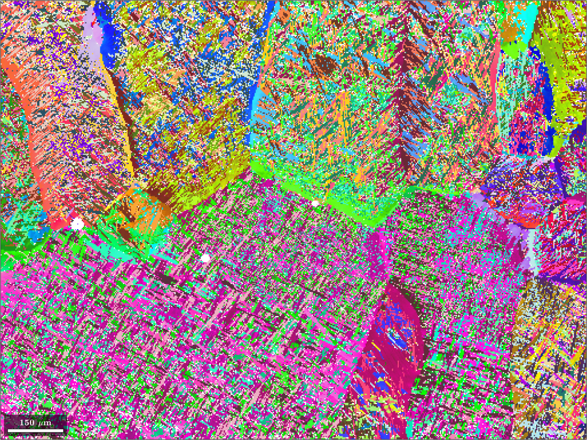

The data set contains 99.8 percent alpha titanium and 0.2 percent beta titanium. Our goal is to reconstuct the original beta phase. The original grain structure appears almost visible for human eyes. Our computations will be based on the Burgers orientation relationship

beta2alpha = orientation.Burgers(ebsd('Ti (beta)').CS,ebsd('Ti (alpha)').CS)

beta2alpha = misorientation (Ti (BETA) → Ti (alpha))
 
 (110) || (0001)   [1-11] || [-2110]

that alligns (110) plane of the beta phase with the (0001) plane of the alpha phase and the [1-11] direction of the beta phase with the [2110] direction of the alpha phase.

Note that all MTEX functions for parent grain reconstruction expect the orientation relationship as parent to child and not as child to parent.

Setting up the parent grain reconstructor

Grain reconstruction is guided in MTEX by a variable of type parentGrainReconstructor. During the reconstruction process this class keeps track about the relationship between the measured child grains and the recovered parent grains. In order to set this variable up we first need to compute the initital child grains from out EBSD data set.

% reconstruct grains
[grains,ebsd.grainId] = calcGrains(ebsd('indexed'),'threshold',1.5*degree,...
  'removeQuadruplePoints');

As our reconstruction will be based on triple junctions we compute the child grains using the option removeQuadruplePoints which turns all quadruple junctions into 2 triple junctions. Furthermore, we choose a very small threshold of 1.5 degree for the identification of grain boundaries to avoid alpha orientations that belong to different beta grains get merged into the same alpha grain.

Now we are ready to set up the parent grain reconstruction job.

job = parentGrainReconstructor(ebsd, grains);

% set the parent to child orientation relationship
job.p2c = beta2alpha

job = parentGrainReconstructor
 
 phase   mineral     symmetry  grains  area   reconstructed
 parent  Ti (BETA)   432       430     0.23%  0%           
 child   Ti (alpha)  622       49120   100%                
 
 OR: (110) || (0001)   [1-11] || [-2110]
   p2c fit: 0.83°, 1.2°, 1.7°, 3.2° (quintiles)
   c2c fit: 0.7°, 0.99°, 1.3°, 1.7° (quintiles)

Compute parent orientations from triple junctions

In present datas set we have very little and unreliable parent measurements. Therefore, we use triple junctions as germ cells for the parent parent grains. In a first step we identify triple junctions that have misorientations that are compatible with a common parent orientation using the command calcTPVotes. The option 'minFit' tells the MTEX that the only those triple junctions are considered where the fit to the common parent orientation does not exceed 2.5 degree.

job.calcTPVotes('minFit',2.5*degree,'maxFit',5*degree)

ans = parentGrainReconstructor
 
 phase   mineral     symmetry  grains  area   reconstructed
 parent  Ti (BETA)   432       430     0.23%  0%           
 child   Ti (alpha)  622       49120   100%                
 
 OR: (110) || (0001)   [1-11] || [-2110]
   p2c fit: 0.83°, 1.2°, 1.7°, 3.2° (quintiles)
   c2c fit: 0.7°, 0.98°, 1.3°, 1.7° (quintiles)
 
 votes: 41427 x 1
   probabilities: 93%, 88%, 82%, 69% (quintiles)

The above command does not only compute the best fitting but also the second best fitting parent orientation. This allows us to ignore ambigues triple points which may vote equally well for different parent orientations. In the above command we did this by the option 'maxFit' which tells MTEX to ignore all triple points where the fit to the second best parent orientation is below 5 degree.

From all remaining triple points the command calcTPVotes compute a list of votes stored in job.votes that contain for each child grain the most likely parent orientation and a corresponding probability job.votes.prob. We may visualize this probability for each grain

plot(job.grains, job.votes.prob(:,1))
mtexColorbar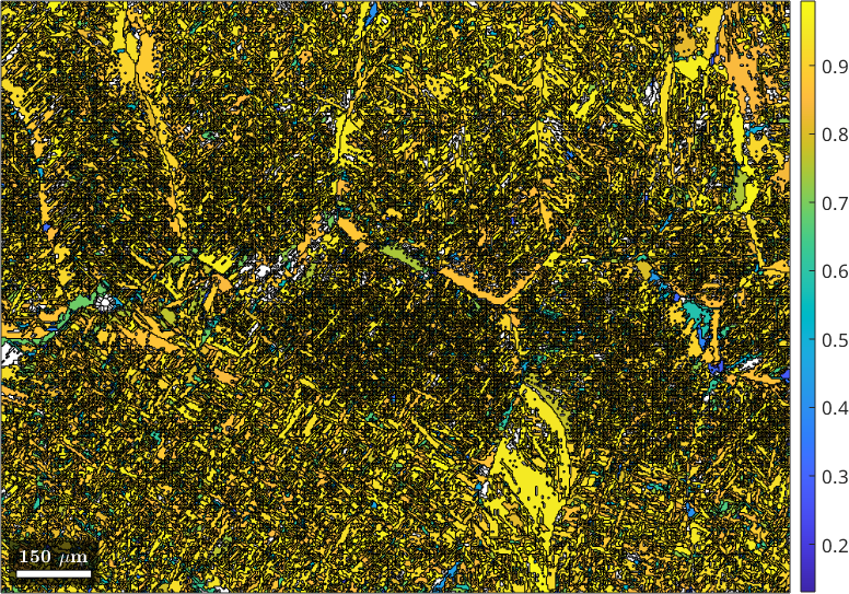

We observe that for most of the grains the probability is above 70 percent. We may use this percentage as threshold to decide which child grains we turn into parent grains. This can be done by the command command calcParentFromVote

job.calcParentFromVote('minProb',0.7)

ans = parentGrainReconstructor
 
 phase   mineral     symmetry  grains  area  reconstructed
 parent  Ti (BETA)   432       33307   84%   67%          
 child   Ti (alpha)  622       16243   16%                
 
 OR: (110) || (0001)   [1-11] || [-2110]
   p2c fit: 0.95°, 1.4°, 1.8°, 2.3° (quintiles)
   c2c fit: 1°, 1.6°, 2°, 2.8° (quintiles)
 
 votes: 8550 x 1
   probabilities: 66%, 61%, 54%, 43% (quintiles)

We observe that after this step more then 66 percent of the grains became parent grains. Lets visualize these reconstructed beta grains

% define a color key
ipfKey = ipfColorKey(ebsd('Ti (Beta)'));
ipfKey.inversePoleFigureDirection = vector3d.Y;

% plot the result
color = ipfKey.orientation2color(job.parentGrains.meanOrientation);
plot(job.parentGrains, color, 'figSize', 'large')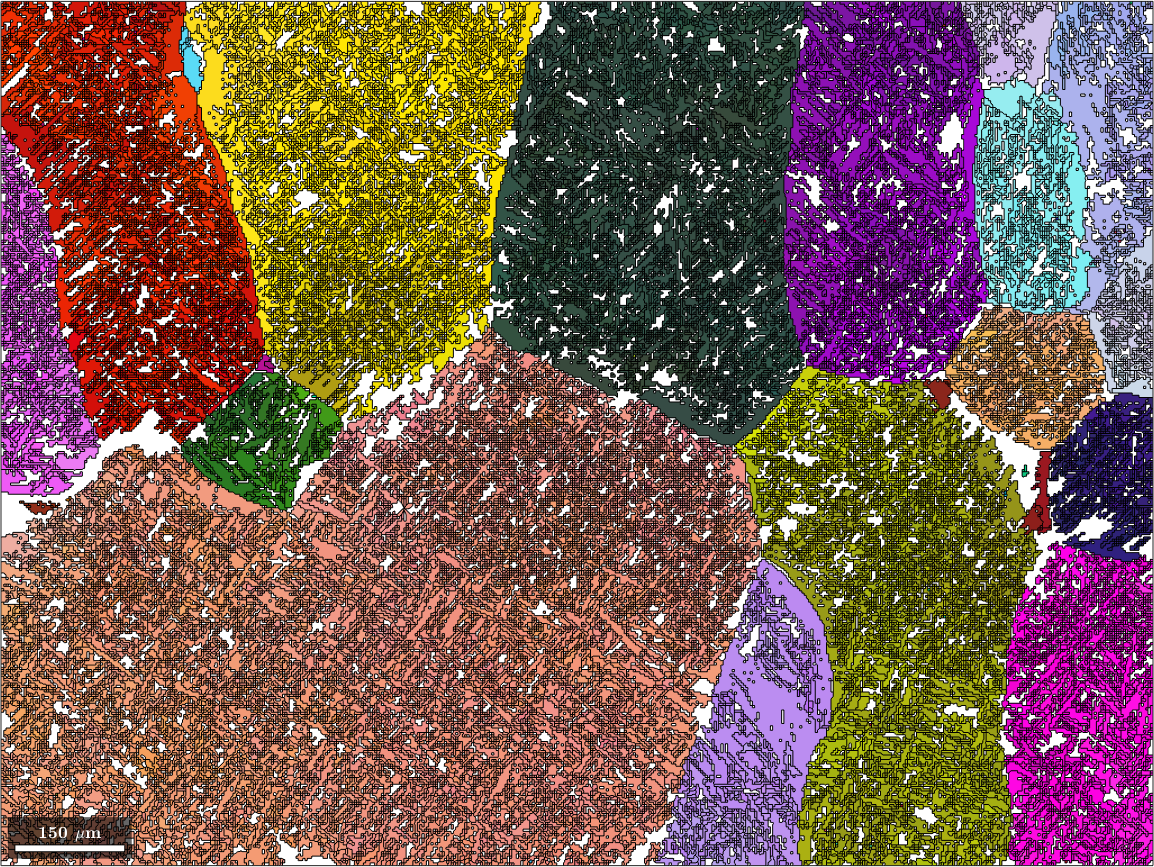

Grow parent grains at grain boundaries

Next we may grow the reconstructed parent grains into the regions of the remaining child grains. To this end we use the command calcGBVotes with the option 'p2c' to compute votes from parent to child grain boundaries. Next we use the exact same command calcParentFromVote to recover parent orientations from the votes. As threshold for the growing the parent grains into the child grains we use 2.5 degree, 5 degree and 7.5 degree. This can be easily accomblished by the following small loop.

for k = 1:3
  job.calcGBVotes('p2c','threshold',k * 2.5*degree);
  job.calcParentFromVote
end

% plot the result
color = ipfKey.orientation2color(job.parentGrains.meanOrientation);
plot(job.parentGrains, color, 'figSize', 'large')

ans = parentGrainReconstructor
 
 phase   mineral     symmetry  grains  area  reconstructed
 parent  Ti (BETA)   432       47995   99%   97%          
 child   Ti (alpha)  622       1555    1%                 
 
 OR: (110) || (0001)   [1-11] || [-2110]
   p2c fit: 16°, 34°, 39°, 42° (quintiles)
   c2c fit: 1.5°, 2.8°, 11°, 25° (quintiles)
 
 votes: 2 x 1
   probabilities: 0%, 0%, 0%, 0% (quintiles)
 
 
ans = parentGrainReconstructor
 
 phase   mineral     symmetry  grains  area   reconstructed
 parent  Ti (BETA)   432       48440   99%    98%          
 child   Ti (alpha)  622       1110    0.66%               
 
 OR: (110) || (0001)   [1-11] || [-2110]
   p2c fit: 33°, 35°, 41°, 42° (quintiles)
   c2c fit: 2.1°, 9.9°, 19°, 25° (quintiles)
 
 votes: 2 x 1
   probabilities: 0%, 0%, 0%, 0% (quintiles)
 
 
ans = parentGrainReconstructor
 
 phase   mineral     symmetry  grains  area   reconstructed
 parent  Ti (BETA)   432       48458   99%    98%          
 child   Ti (alpha)  622       1092    0.65%               
 
 OR: (110) || (0001)   [1-11] || [-2110]
   p2c fit: 34°, 35°, 41°, 42° (quintiles)
   c2c fit: 1.6°, 9.2°, 19°, 29° (quintiles)
 
 votes: 2 x 1
   probabilities: 0%, 0%, 0%, 0% (quintiles)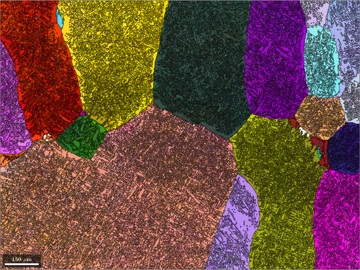

Merge parent grains

After the previous steps we are left with many very similar parent grains. In order to merge all similarly oriented grains into large parent grains one can use the command mergeSimilar. It takes as an option the threshold below which two parent grains should be considered a a single grain.

job.mergeSimilar('threshold',5*degree)

% plot the result
color = ipfKey.orientation2color(job.parentGrains.meanOrientation);
plot(job.parentGrains, color, 'figSize', 'large')

ans = parentGrainReconstructor
 
 phase   mineral     symmetry  grains  area   reconstructed
 parent  Ti (BETA)   432       155     99%    98%          
 child   Ti (alpha)  622       1074    0.65%               
 
 OR: (110) || (0001)   [1-11] || [-2110]
   p2c fit: 33°, 35°, 41°, 42° (quintiles)
   c2c fit: 9.2°, 18°, 19°, 25° (quintiles)
 
 votes: 2 x 1
   probabilities: 0%, 0%, 0%, 0% (quintiles)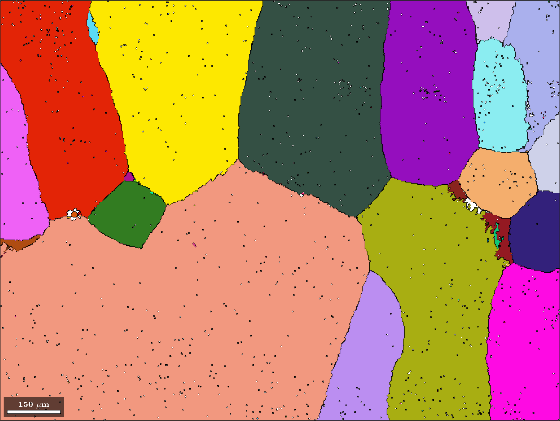

Merge inclusions

We may be still a bit unsatisfied with the result as the large parent grains contain a lot of poorly indexed inclusions where we failed to assign a parent orientation. We use the command mergeInclusions to merge all inclusions that have fever pixels then a certain threshold into the surrounding parent grains.

job.mergeInclusions('maxSize',5)

% plot the result
color = ipfKey.orientation2color(job.parentGrains.meanOrientation);
plot(job.parentGrains, color, 'figSize', 'large')

ans = parentGrainReconstructor
 
 phase   mineral     symmetry  grains  area    reconstructed
 parent  Ti (BETA)   432       66      100%    100%         
 child   Ti (alpha)  622       70      0.093%               
 
 OR: (110) || (0001)   [1-11] || [-2110]
   p2c fit: 23°, 29°, 33°, 35° (quintiles)
   c2c fit: 4.1°, 9.8°, 19°, 32° (quintiles)
 
 votes: 2 x 1
   probabilities: 0%, 0%, 0%, 0% (quintiles)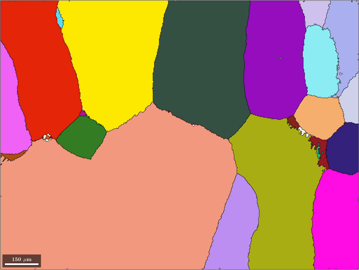

Reconstruct beta orientations in EBSD map

Until now we have only recovered the beta orientations as the mean orientations of the beta grains. In this section we want to set up the EBSD variable parentEBSD to contain for each pixel a reconstruction of the parent phase orientation. This is done by the command calcParentEBSD

parentEBSD = job.ebsd;

% plot the result
color = ipfKey.orientation2color(parentEBSD('Ti (Beta)').orientations);
plot(parentEBSD('Ti (Beta)'),color,'figSize','large')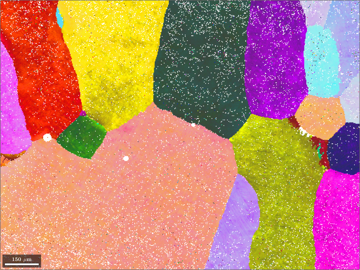

The recovered EBSD variable parentEBSD contains a measure parentEBSD.fit for the corespondence between the beta orientation reconstructed for a single pixel and the beta orientation of the grain. Lets visualize this

% the beta phase
plot(parentEBSD, parentEBSD.fit ./ degree,'figSize','large')
mtexColorbar
setColorRange([0,5])
mtexColorMap('LaboTeX')

hold on
plot(job.grains.boundary,'lineWidth',2)
hold off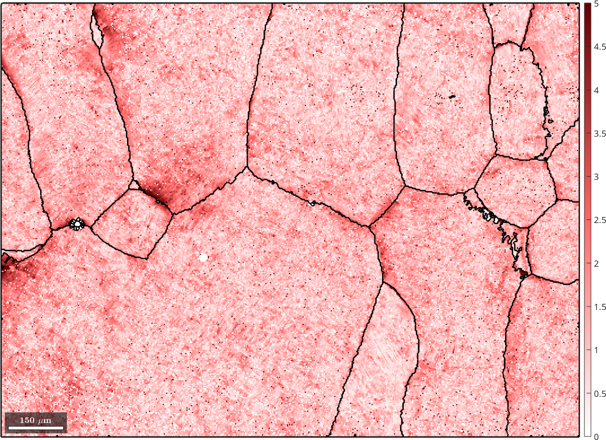

For comparison the map with original alpha phase and on top the recovered beta grain boundaries

plot(ebsd('Ti (Alpha)'),ebsd('Ti (Alpha)').orientations,'figSize','large')

hold on
parentGrains = smooth(job.grains,5);
plot(parentGrains.boundary,'lineWidth',3)
hold off