Fundamental Regions

Fundamental Regions edit page

Thanks to crystal symmetry the space of all rotations can be reduced to a so called fundamental or asymmetric region which has the property that each for orientation there is "exactly" one symmetrically equivalent orientation that is within the fundamental region. Those regions play an important role for visualizing orientations and ODFs as well as for the computation of axis and angle distributions of misorientations.

The space of all orientations can be imagined as a three dimensional ball with radius 180 degree. The distance of some point in the ball to the origin represent the rotational angle and the vector represents the rotational axis. In MTEX this can be represented as follows

% triclinic crystal symmetry
cs = crystalSymmetry('triclinic')

% the corresponding orientation space
oR_all = fundamentalRegion(cs);

% lets plot the ball of all orientations
plot(oR_all)

cs = crystalSymmetry
 
  symmetry          : -1                 
  elements          : 2                  
  a, b, c           : 1, 1, 1            
  alpha, beta, gamma: 90°, 90°, 90°      
  reference frame   : X||a*, Y||b*, Z||c*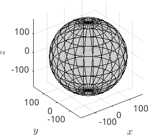

Next we plot some orientations into this space

% rotation about the z-axis about 180 degree
rotZ = orientation.byAxisAngle(zvector,180*degree,cs);

hold on
plot(rotZ,'MarkerColor','b','MarkerSize',10)
hold off

% rotations about the x- and y-axis about 30,60,90 ... degree
rotX = orientation.byAxisAngle(xvector,(-180:30:180)*degree,cs);
rotY = orientation.byAxisAngle(yvector,(-180:30:180)*degree,cs);

hold on
plot(rotX,'MarkerColor','r','MarkerSize',10)
plot(rotY,'MarkerColor','g','MarkerSize',10)
hold off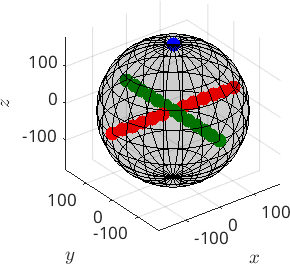

An alternative view on the orientation space is by sections, e.g. sections along the Euler angles or along the rotational angle. The latter one should be demonstrated next:

plotSection(rotZ,'MarkerColor','b','axisAngle',(30:30:180)*degree)
hold on
plot(rotX,'MarkerColor','g','add2all')
hold on
plot(rotY,'MarkerColor','r','add2all')
hold off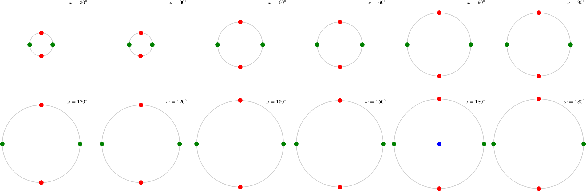

Crystal Symmetries

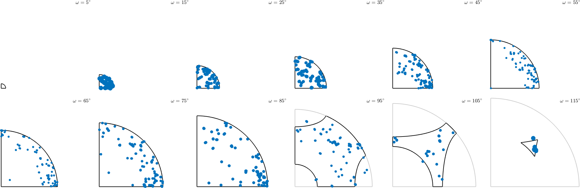
In case of crystal symmetries the orientation space can divided into as many equivalent segments as the symmetry group has elements. E.g. in the case of orthorhombic symmetry the orientation space is subdivided into four equal parts, the central one looking like

cs = crystalSymmetry('222')
oR = fundamentalRegion(cs);

close all
plot(oR_all)
hold on
plot(oR,'color','r')
hold off

cs = crystalSymmetry
 
  symmetry: 222    
  elements: 4      
  a, b, c : 1, 1, 1
 
Warning: Possible symmetry mismach!

As an example consider the following EBSD data set

mtexdata forsterite

ebsd = EBSD
 
 Phase  Orientations     Mineral         Color  Symmetry  Crystal reference frame
     0   58485 (24%)  notIndexed                                                 
     1  152345 (62%)  Forsterite  LightSkyBlue       mmm                         
     2   26058 (11%)   Enstatite  DarkSeaGreen       mmm                         
     3   9064 (3.7%)    Diopside     Goldenrod     12/m1       X||a*, Y||b*, Z||c
 
 Properties: bands, bc, bs, error, mad, x, y
 Scan unit : um

we can visualize the Forsterite orientations by

plot(ebsd('Fo').orientations,'axisAngle')

plot 2000 random orientations out of 152345 given orientations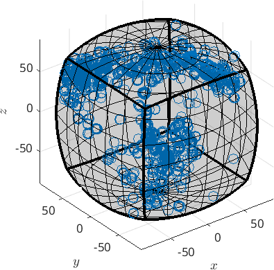

We see that all orientations are automatically projected inside the fundamental region. In order to compute explicitly the represent inside the fundamental region we can do

ori =  ebsd('Fo').orientations.project2FundamentalRegion

ori = orientation (Forsterite → xyz)
  size: 152345 x 1

Change the center of the fundamental region

There is no necessity that the fundamental region has to be centered in the origin - it can be centered at any orientation, e.g. at the mean orientation of a grain.

% segment data into grains
[grains,ebsd.grainId] = calcGrains(ebsd('indexed'));

% take the orientations of the largest on
[~,id] = max(grains.area);
largeGrain = grains(id)
ori = ebsd(largeGrain).orientations

% recenter the fundamental zone to the mean orientation
center = largeGrain.meanOrientation;
plot(rotate(oR,center))

% project the orientations into the fundamental region around the mean
% orientation
ori = ori.project2FundamentalRegion(center)

hold on
plot(ori,'axisAngle')
hold off

largeGrain = grain2d
 
 Phase  Grains  Pixels     Mineral  Symmetry  Crystal reference frame
     1       1    2683  Forsterite       mmm                         
 
 boundary segments: 714 (32000 µm)
 inner boundary segments: 0 (0 µm)
 triple points: 44
 
  Id   Phase   Pixels   phi1   Phi   phi2         GOS
 931       1     2683    171    55    261   0.0441053
 
 
ori = orientation (Forsterite → xyz)
  size: 2683 x 1
 
ori = orientation (Forsterite → xyz)
  size: 2683 x 1
 
 
cs1 = crystalSymmetry
 
  mineral : Forsterite  
  color   : LightSkyBlue
  symmetry: mmm         
  elements: 8           
  a, b, c : 4.8, 10, 6  
 
 
cs2 = crystalSymmetry
 
  symmetry: 222    
  elements: 4      
  a, b, c : 1, 1, 1
 
plot 2000 random orientations out of 2683 given orientations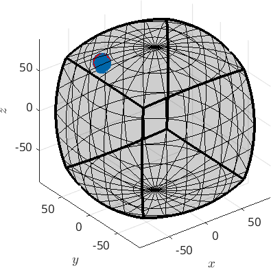

Fundamental regions of misorientations

Misorientations are characterized by two crystal symmetries. A corresponding fundamental region is defined by

oR = fundamentalRegion(ebsd('Fo').CS,ebsd('En').CS);

plot(oR)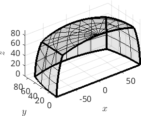

Let plot grain boundary misorientations within this fundamental region

plot(grains.boundary('fo','En').misorientation)

plot 2000 random orientations out of 11814 given orientations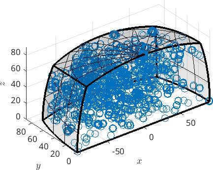

Fundamental regions of misorientations with antipodal symmetry

Note that for boundary misorientations between the same phase we can not distinguish between a misorientation and its inverse. This is not the case for misorientations between different phases or the misorientation between the mean orientation of a grain and all other orientations. The inverse of a misorientation is axis - angle representation is simply the one with the same angle but antipodal axis. Accordingly this additional symmetry is handled in MTEX by the keyword 'antipodal'.

oR = fundamentalRegion(ebsd('Fo').CS,ebsd('Fo').CS,'antipodal');

plot(oR)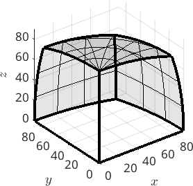

We see that the fundamental region with antipodal symmetry has only half the size as without. In the case of misorientations between the same phase MTEX automatically sets the flag 'antipodal' to the misorientations and plots them accordingly.

mori = grains.boundary('Fo','Fo').misorientation
plot(mori)

mori = misorientation (Forsterite → Forsterite)
  size: 15974 x 1
  antipodal:         true
plot 2000 random orientations out of 15974 given orientations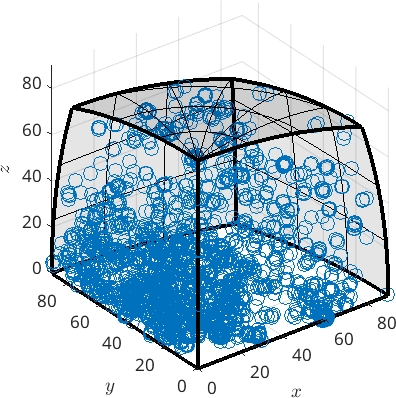

If you want to avoid this you can remove the flag 'antipodal' by

mori.antipodal = false;

plot(mori)

plot 2000 random orientations out of 15974 given orientations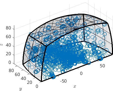

Axis angle sections

Again we can plot constant angle sections through the fundamental region. This is done by

plotSection(mori,'axisAngle')

plotting 2000 random orientations out of 15974 given orientations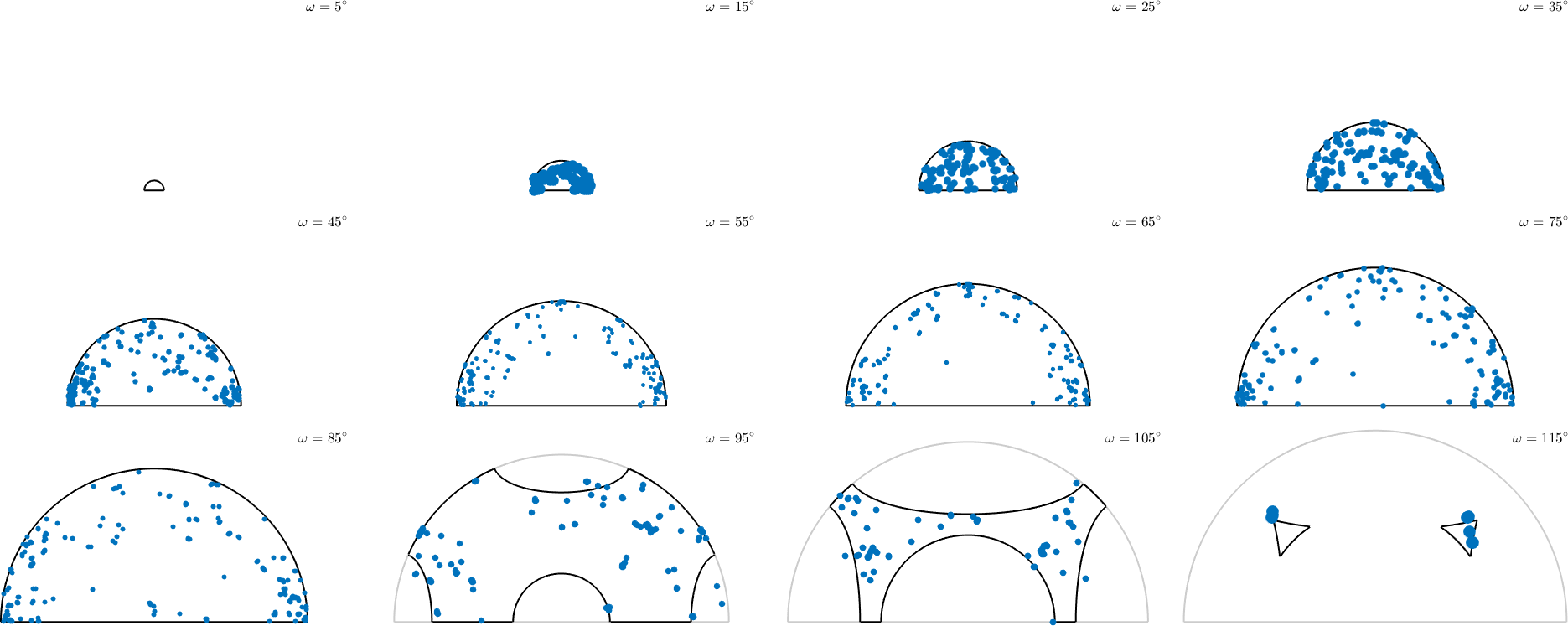

Note that in the previous plot we distinguish between mori and inv(mori). Adding antipodal symmetry those are considered as equivalent

plotSection(mori,'axisAngle','antipodal')

%
%
%<html>
%   <div class="note">
%      <b>ok&lt;*NASGU&gt;
%</b>
%      <text/>
%   </div>
%</html>
%

plotting 2000 random orientations out of 15974 given orientations