In this section we consider the analysis of twining. Therefore lets start by importing some Magnesium data and reconstructing the grain structure.
% load some example data
mtexdata twins

% segment grains
[grains,ebsd.grainId,ebsd.mis2mean] = calcGrains(ebsd('indexed'),...
  'angle',5*degree,'minPixel',3);

% smooth them
grains = grains.smooth(5);

% visualize the grains
plot(grains,grains.meanOrientation)

% store crystal symmetry of Magnesium
CS = grains.CS;
ebsd = EBSD (y↑→x)
Phase Orientations Mineral Color Symmetry Crystal reference frame
0 46 (0.2%) notIndexed
1 22833 (100%) Magnesium LightSkyBlue 6/mmm X||a*, Y||b, Z||c*
Properties: bands, bc, bs, error, mad
Scan unit : um
X x Y x Z : [0, 50] x [0, 41] x [0, 0]
Normal vector: (0,0,1)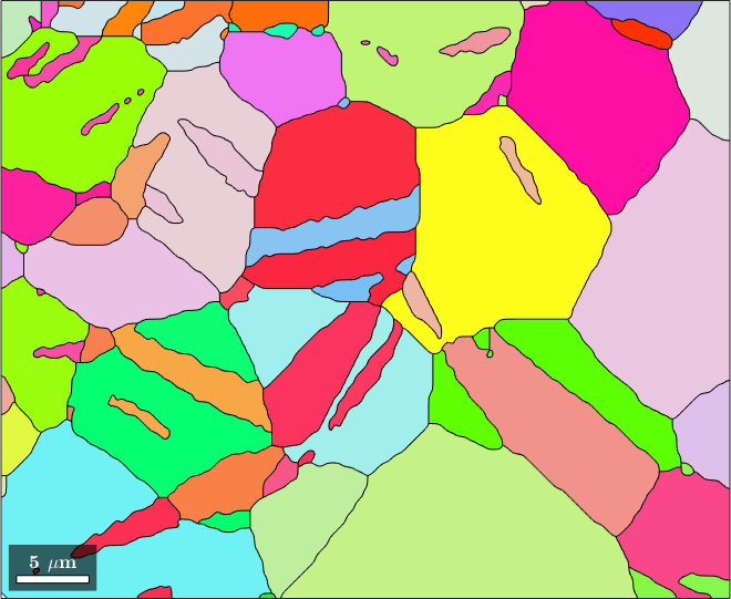
Next we extract the grain boundaries and save them to a separate variable
gB = grains.boundarygB = grainBoundary
Segments length mineral 1 mineral 2
1181 184 µm notIndexed Magnesium
3164 724 µm Magnesium MagnesiumThe output tells us that we have 3219 Magnesium to Magnesium boundary segments and 606 boundary segments where the grains are cut by the scanning boundary. To restrict the grain boundaries to a specific phase transition you shall do
gB_MgMg = gB('Magnesium','Magnesium')gB_MgMg = grainBoundary
Segments length mineral 1 mineral 2
3164 724 µm Magnesium MagnesiumProperties of grain boundaries
A variable of type grain boundary contains the following properties
- misorientation
- direction
- segLength
These can be used to colorize the grain boundaries. By the following command, we plot the grain boundaries colorized by the misorientation angle
plot(gB_MgMg,gB_MgMg.misorientation.angle./degree,'linewidth',2)
mtexColorbar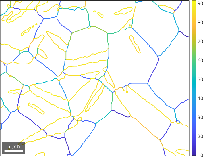
We observe that we have many grain boundaries with misorientation angle larger than 80 degree. In order to investigate the distribution of misorientation angles further we have the look at a misorientation angle histogram.
close all
histogram(gB_MgMg.misorientation.angle./degree,40)
xlabel('misorientation angle (degree)')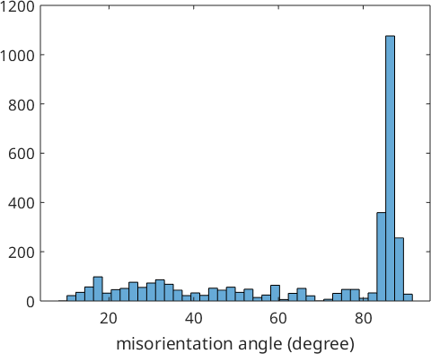
Lets analyze the misorientations corresponding to the peak around 86 degree in more detail. Therefore, we consider only those misorientations with misorientation angle between 85 and 87 degree
ind = gB_MgMg.misorientation.angle>85*degree & gB_MgMg.misorientation.angle<87*degree;
mori = gB_MgMg.misorientation(ind);
and observe that when plotted in axis angle domain they form a strong cluster close to one of the corners of the domain.
scatter(mori)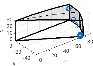
We may determine the center of the cluster and check whether it is close to some special orientation relation ship
% determine the mean of the cluster
mori_mean = mean(mori,'robust')

% determine the closest special orientation relation ship
round2Miller(mori_mean)
mori_mean = misorientation (Magnesium → Magnesium)
antipodal: true
Bunge Euler angles in degree
phi1 Phi phi2
29.9378 93.904 30.4111
plane parallel direction parallel fit
(11̅01) || (101̅1̅) [011̅1] || [11̅01] 0.466°Bases on the output above we may now define the special orientation relationship as
twinning = orientation.map(Miller(1,-1,0,1,CS),Miller(1,0,-1,-1,CS),...
  Miller(0,1,-1,1,CS,'uvw'),Miller(1,-1,0,1,CS,'uvw'))
twinning = misorientation (Magnesium → Magnesium)
(101̅1̅) || (011̅1) [011̅1] || [11̅01]Considering the disorientation angle we observe that it is 86.3 degree with respect to the axis (-1210)
% the rotational axis
round(twinning.axis)

% the rotational angle
twinning.angle / degree
ans = Miller (Magnesium)
h k i l
1 1 -2 0
ans =
86.2992However, remembering that twinning refers to rotations about 180 degrees we may ask for the symmetrically equivalent misorientation with the maximum misorientation angle. This can be computed using the option 'max'
angle(twinning,'max')/degreeans =
180The corresponding rotational axis is
v = round(Miller(axis(twinning,'max'),'UVTW'))v = Miller (Magnesium)
U V T W
2 0 -2 1Next, we check for each boundary segment whether it is a twinning boundary, i.e., whether boundary misorientation is close to the twinning.
% restrict to twinnings with threshold 5 degree
isTwinning = angle(gB_MgMg.misorientation,twinning) < 5*degree;
twinBoundary = gB_MgMg(isTwinning)

% plot the twinning boundaries
plot(grains,grains.meanOrientation)
%plot(ebsd('indexed'),ebsd('indexed').orientations)
hold on
%plot(gB_MgMg,angle(gB_MgMg.misorientation,twinning),'linewidth',4)
plot(twinBoundary,'linecolor','w','linewidth',4,'displayName','twin boundary')
hold off
twinBoundary = grainBoundary
Segments length mineral 1 mineral 2
1649 361 µm Magnesium Magnesium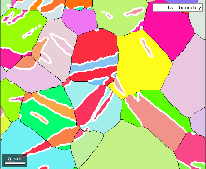
A common next step is to reconstruct the grain structure parent to twinning by merging the twinned grains. This is explained in detail in the section Merging Grains.