In this section we discuss specific operations that are available for EBSD data which are measured on a square or hexagonal grid.
By default MTEX ignores any gridding in the data. The reason for this is that when restricting to some subset, e.g. to a certain phase, the data will not form a regular grid anyway. For that reason, almost all functions in MTEX are implemented to work for arbitrarily aligned data.
On the other hand, there are certain functions that are only available or much faster for gridded data. Those functions include plotting, gradient computation and denoising. The key command to make MTEX aware of EBSD data on a hexagonal or square grid is gridify.
In order to explain the corresponding concept in more detail lets import some sample data.
mtexdata twins

plot(ebsd('Magnesium'),ebsd('Magnesium').orientations)
ebsd = EBSD (y↑→x)
Phase Orientations Mineral Color Symmetry Crystal reference frame
0 46 (0.2%) notIndexed
1 22833 (100%) Magnesium LightSkyBlue 6/mmm X||a*, Y||b, Z||c*
Properties: bands, bc, bs, error, mad
Scan unit : um
X x Y x Z : [0, 50] x [0, 41] x [0, 0]
Normal vector: (0,0,1)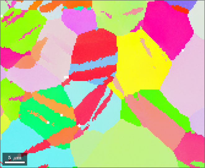
As we can see already from the phase plot above the data have been measured at an rectangular grid. A quick look at the unit cell verifies this
ebsd.unitCellans = vector3d (y↑→x)
size: 4 x 1
x y z
0.15 0.15 0
-0.15 0.15 0
-0.15 -0.15 0
0.15 -0.15 0If we apply the command gridify to the data set
ebsd = ebsd.gridifyebsd = EBSDsquare (y↑→x)
Phase Orientations Mineral Color Symmetry Crystal reference frame
0 46 (0.2%) notIndexed
1 22833 (100%) Magnesium LightSkyBlue 6/mmm X||a*, Y||b, Z||c*
Properties: bands, bc, bs, error, mad, oldId
Scan unit : um
X x Y x Z : [0, 50] x [0, 41] x [0, 0]
Normal vector: (0,0,1)
Square grid :137 x 167we data get aligned in a 137 x 167 matrix. In particular we may now apply standard matrix indexing to our EBSD data, e.g., to access the EBSD data at position 50,100 we can simply do
ebsd(50,100)ans = EBSD (y↑→x)
Phase Orientations Mineral Color Symmetry Crystal reference frame
1 1 (100%) Magnesium LightSkyBlue 6/mmm X||a*, Y||b, Z||c*
Id Phase orientation bands bc bs error mad oldId
13613 1 (155.8°,100.6°,239.3°) 10 149 133 0 0.7 8283
Scan unit : um
X x Y x Z : [30, 30] x [15, 15] x [0, 0]
Normal vector: (0,0,1)It is important to understand that the property of being shaped as a matrix is lost as soon as we select a subset of data
ebsdMg = ebsd('Magnesium')ebsdMg = EBSD (y↑→x)
Phase Orientations Mineral Color Symmetry Crystal reference frame
1 22833 (100%) Magnesium LightSkyBlue 6/mmm X||a*, Y||b, Z||c*
Properties: bands, bc, bs, error, mad, oldId
Scan unit : um
X x Y x Z : [0, 50] x [0, 41] x [0, 0]
Normal vector: (0,0,1)However, we may always force it into matrix form by reapplying the command gridify
ebsdMg = ebsd('Magnesium').gridifyebsdMg = EBSDsquare (y↑→x)
Phase Orientations Mineral Color Symmetry Crystal reference frame
1 22833 (100%) Magnesium LightSkyBlue 6/mmm X||a*, Y||b, Z||c*
Properties: bands, bc, bs, error, mad, oldId
Scan unit : um
X x Y x Z : [0, 50] x [0, 41] x [0, 0]
Normal vector: (0,0,1)
Square grid :137 x 167The difference between both matrix shapes EBSD variables ebsd and ebsdMg is that not indexed pixels in ebsd are stored as the separate phase 'notIndexed' while in ebsdMg all pixels have phase Magnesium but the Euler angles of the not indexed pixels are set to nan. This allows to select and plot subregions of the EBSD map in a very intuitive way by
plot(ebsdMg(50:100,5:100),ebsdMg(50:100,5:100).orientations)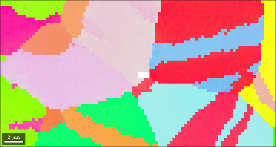
The Gradient
Data on a square or hexagonal grid has the additional advantage to allow the computation of the orientations gradient, the incomplete Nye tensor, as well the weighted Burgers vector.
gradX = ebsdMg.gradientX;

plot(ebsdMg,norm(gradX))
setColorRange([0,4*degree])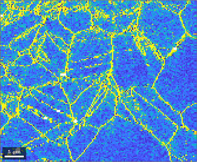
Hexagonal Grids
Next lets import some data on a hexagonal grid
mtexdata copper silent

[grains, ebsd.grainId] = calcGrains(ebsd);
ebsd = ebsd.gridify

plot(ebsd,ebsd.orientations)
ebsd = EBSDhex (y↑→x)
Phase Orientations Mineral Color Symmetry Crystal reference frame
0 16116 (100%) Copper LightSkyBlue 432
Properties: confidenceindex, fit, imagequality, semsignal, unknown_11, unknown_12, unknown_13, unknown_14, grainId, oldId
Scan unit : um
X x Y x Z : [0, 593] x [0, 585] x [0, 0]
Normal vector: (0,0,1)
Hex grid :136 x 119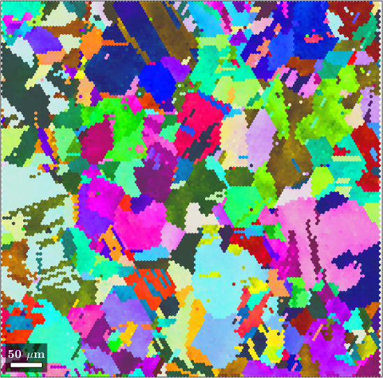
Indexing works here similarly as for square grids
plot(ebsd(1:20,1:40),ebsd(1:20,1:40).orientations,'micronbar','off','edgeColor','black')
Switching from Hexagonal to Square Grid
Sometimes it is required to resample EBSD data on a hex grid on a square grid. This can be accomplished by passing to the command gridify a square unit cell by the option unitCell.
% define a square unit cell
unitCell = 2.5 * vector3d([-1 -1 1 1].',[-1 1 1 -1].',0);

% use the square unit cell for gridify
ebsdS = ebsd.gridify('unitCell',unitCell)

% visualize the result
plot(ebsd,ebsd.orientations,'layout',[1,2])
nextAxis
plot(ebsdS, ebsdS.orientations)
ebsdS = EBSDsquare (y↑→x)
Phase Orientations Mineral Color Symmetry Crystal reference frame
-1 139 (0.98%) notIndexed
0 14021 (99%) Copper LightSkyBlue 432
Properties: confidenceindex, fit, imagequality, semsignal, unknown_11, unknown_12, unknown_13, unknown_14, grainId, oldId
Scan unit : um
X x Y x Z : [0, 595] x [0, 585] x [0, 0]
Normal vector: (0,0,1)
Square grid :118 x 120
In the above example we have chosen the square unit cell to have approximately the same size as the hexagonal unit cell. This leads to quite some distortions as squares can not reproduces all the shapes of the hexagons. We can reduce this issue by choosing the square unit cell significantly smaller then the hexagonal unit cell.
% a smaller unit cell
unitCell = 0.5*vector3d([-1 -1 1 1].',[-1 1 1 -1].',0);

% use the small square unit cell for gridify
ebsdS = ebsd.gridify('unitCell',unitCell)
nextAxis
plot(ebsdS,ebsdS.orientations)
hold on
plot(grains.boundary,'lineWidth',2)
hold off
ebsdS = EBSDsquare (y↑→x)
Phase Orientations Mineral Color Symmetry Crystal reference frame
-1 1310 (0.38%) notIndexed
0 346774 (100%) Copper LightSkyBlue 432
Properties: confidenceindex, fit, imagequality, semsignal, unknown_11, unknown_12, unknown_13, unknown_14, grainId, oldId
Scan unit : um
X x Y x Z : [0, 593] x [0, 585] x [0, 0]
Normal vector: (0,0,1)
Square grid :586 x 594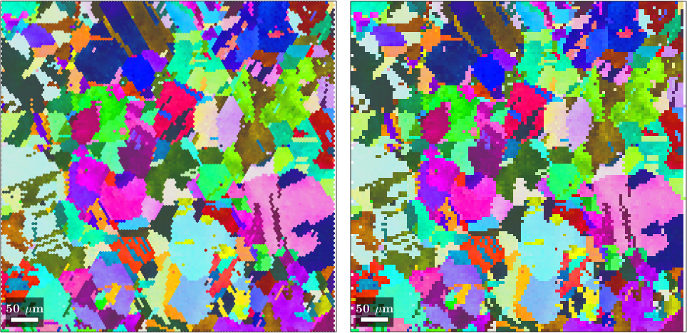
It is important to understand that the command gridify does not increase the number of data points. As a consequence, we end up with many white spots in the map which corresponds to orientations that have been set to NaN. In order to fill these white spots, we may either use the command fill which performs nearest neighbor interpolation or the command smooth which allows for more sophisticated interpolation methods.
% nearest neighbor interpolation
ebsdS1 = fill(ebsdS,grains)

plot(ebsdS1('indexed'),ebsdS1('indexed').orientations)
hold on
plot(grains.boundary,'lineWidth',2)
hold off
ebsdS1 = EBSDsquare (y↑→x)
Phase Orientations Mineral Color Symmetry Crystal reference frame
-1 1310 (0.38%) notIndexed
0 346774 (100%) Copper LightSkyBlue 432
Properties: confidenceindex, fit, imagequality, semsignal, unknown_11, unknown_12, unknown_13, unknown_14, grainId, oldId
Scan unit : um
X x Y x Z : [0, 593] x [0, 585] x [0, 0]
Normal vector: (0,0,1)
Square grid :586 x 594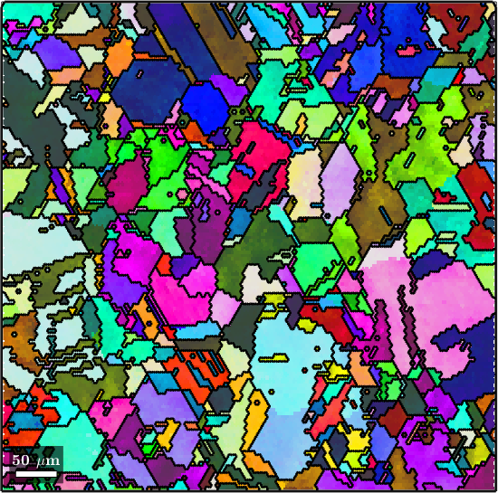
% interpolation using a TV regularization term
F = halfQuadraticFilter;
F.alpha = 0.5;
ebsdS2 = smooth(ebsdS,F,'fill',grains)

nextAxis(1,2)
plot(ebsdS2('indexed'),ebsdS2('indexed').orientations)
hold on
plot(grains.boundary,'lineWidth',2)
hold off
ebsdS2 = EBSD (y↑→x)
Phase Orientations Mineral Color Symmetry Crystal reference frame
-1 1310 (0.38%) notIndexed
0 346774 (100%) Copper LightSkyBlue 432
Properties: confidenceindex, fit, imagequality, semsignal, unknown_11, unknown_12, unknown_13, unknown_14, grainId, oldId, quality
Scan unit : um
X x Y x Z : [0, 593] x [0, 585] x [0, 0]
Normal vector: (0,0,1)
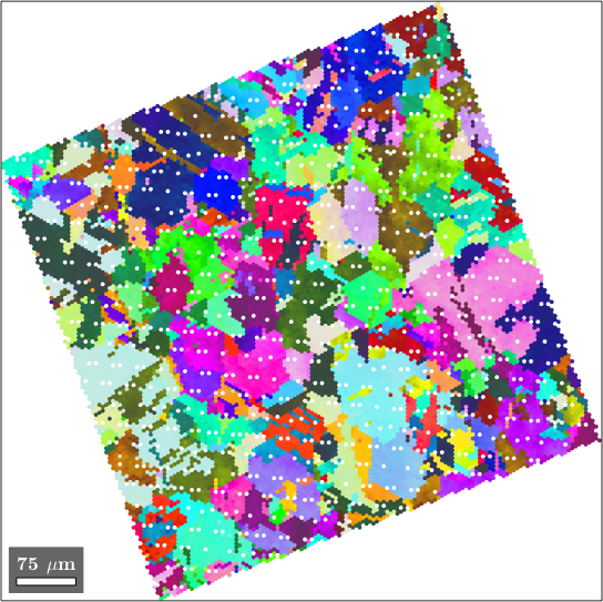
Gridify on Rotated Maps
A similar situation occurs if gridify is applied to rotated data.
ebsd = rotate(ebsd,20*degree);

ebsdG = ebsd.gridify

plot(ebsdG,ebsdG.orientations)
ebsdG = EBSDhex (y↑→x)
Phase Orientations Mineral Color Symmetry Crystal reference frame
0 15302 (58%) Copper LightSkyBlue 432
Properties: confidenceindex, fit, imagequality, semsignal, unknown_11, unknown_12, unknown_13, unknown_14, grainId, oldId
Scan unit : um
X x Y x Z : [-198, 555] x [0, 753] x [0, 0]
Normal vector: (0,0,1)
Hex grid :151 x 175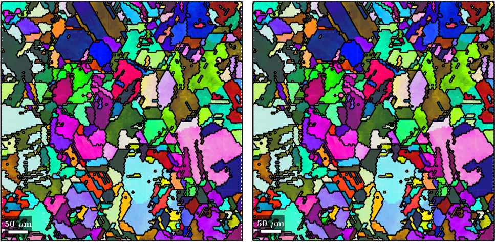
Again we may observe white spots within the map which we can easily fill with the fill command.
ebsdGF = fill(ebsdG)

plot(ebsdGF,ebsdGF.orientations)
ebsdGF = EBSDhex (y↑→x)
Phase Orientations Mineral Color Symmetry Crystal reference frame
0 16210 (61%) Copper LightSkyBlue 432
Properties: confidenceindex, fit, imagequality, semsignal, unknown_11, unknown_12, unknown_13, unknown_14, grainId, oldId
Scan unit : um
X x Y x Z : [-198, 555] x [0, 753] x [0, 0]
Normal vector: (0,0,1)
Hex grid :151 x 175