
extend EBSD data to an grid
Description
In the default column major layout the first dimension of the resulting matrix is the grid direction closest to y and the second one the grid direction closest to x, both oriented such that the coordinates increase. Accordingly ebsd(i,j) is the j-th pixel of the i-th scan row and ebsd(1,1) is the corner with the smallest coordinates. Hexagonal grids are always stored this way, the flags apply to square grids only.
The two flags are the two layouts a gridLayout can state that are aligned with x and y, and any other axis aligned layout may be asked for by handing one over instead - which is how a map is put in the same order as an image it is to be compared with pixel by pixel. A grid that is rotated or sheared cannot land on the requested layout exactly and is put as close to it as a permutation can get.
The layout is a property of the MAP, not of the file: it is the same whichever corner the acquisition started from and whichever direction it scanned in.
Gridding therefore REORDERS the measurements gridify does not preserve the order the measurements arrive in, and cannot: the layout above fixes the first matrix dimension to y, while a .ctf or .ang is written with x varying fastest, so MATLAB's column major linear indexing runs down the map where the file runs across it. The two coincide only for a file that happens to scan y fastest. newId is the translation - ebsdGrid.pos(newId) == ebsd.pos - and ebsdGrid.oldId carries the original ids.
Of the sample files shipped with MTEX, none keeps its order under the default layout and seven of eleven keep it under 'rowMajor'; the rest cannot be matched by either flag, because they scan x descending (Emsland_plessite) or are hexagonal. Reordering is thus the normal case, and 'rowMajor' is a layout choice, not a way to preserve the input order.
This is safe for reconstruction: calcGrains is invariant under the order of its input - shuffling forsterite's 187467 indexed measurements at random reproduces the grain count and the multiset of boundary segment lengths exactly, with the total length moving by 2 ulp from summation order alone. Anything that does depend on the order is a defect in that code rather than a reason to reshape the grid; see latticeBasis, which used to derive a mirrored lattice basis from the reordered unit cell.
Syntax
[ebsdGrid,newId] = gridify(ebsd)
[ebsdGrid,newId] = gridify(ebsd,'unitCell',unitCell)
[ebsdGrid,newId] = gridify(ebsd,'rowMajor')
[ebsdGrid,newId] = gridify(ebsd,gridLayout(otherMap))
Input
| ebsd | an EBSD data set with a non regular grid |
| gL | gridLayout, any axis aligned layout |
Options
| extent | extend of gridded map |
| unitCell | unit cell of the gridded map |
Flags
| columnMajor | one scan row per matrix row, i.e. size(ebsd) = [numRows numCols] (default) |
| rowMajor | the transposed layout, i.e. size(ebsd) = [numCols numRows] |
Output
| ebsd | EBSDsquare, EBSDhex data on a regular grid |
| newId | closest regular grid point for every non regular grid point |
Example
mtexdata twins
ebsdMg = ebsd('Magnesium').gridify
plot(ebsdMg, ebsdMg.orientations)
ebsd = EBSDsquare (y↓→x, row↓→col)
Phase Orientations Mineral Color Symmetry Crystal reference frame
0 46 (0.2%) notIndexed none
1 22833 (100%) Magnesium LightSkyBlue 6/mmm X||a*, Y||b, Z||c
Properties: bands, bc, bs, error, mad, oldId
Scan unit : um
X × Y × Z : [0 → 50] × [0 → 41] × [0 → 0]
Normal vector: (0,0,1)
Square grid :137 × 167
ebsdMg = EBSDsquare (y↓→x, row↓→col)
Phase Orientations Mineral Color Symmetry Crystal reference frame
1 22833 (100%) Magnesium LightSkyBlue 6/mmm X||a*, Y||b, Z||c
Properties: bands, bc, bs, error, mad, oldId
Scan unit : um
X × Y × Z : [0 → 50] × [0 → 41] × [0 → 0]
Normal vector: (0,0,1)
Square grid :137 × 167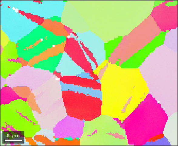
Citing this page.
This page is part of the documentation of
MTEX, a free and open
source MATLAB toolbox for analyzing and modeling crystallographic textures.
It was written by The MTEX Developers and is published at
https://mtex-toolbox.github.io/EBSD.gridify.html.
If you use MTEX, or reuse text or figures from this page, in your research,
please cite
F. Bachmann, R. Hielscher, H. Schaeben: Texture Analysis with MTEX - Free and Open Source Software Toolbox, Solid State Phenomena 160 (2010), 63-68. 10.4028/www.scientific.net/SSP.160.63
BibTeX
@article{bachmann2010mtex,
  author  = {F. Bachmann and R. Hielscher and H. Schaeben},
  title   = {Texture Analysis with MTEX - Free and Open Source Software Toolbox},
  journal = {Solid State Phenomena},
  volume  = {160},
  pages   = {63-68},
  year    = {2010},
  doi     = {10.4028/www.scientific.net/SSP.160.63},
  url     = {https://doi.org/10.4028/www.scientific.net/SSP.160.63}
}
Other papers describing specific MTEX methods are listed under Publications — please cite the one that best fits your application. The MTEX source code is licensed under the GNU General Public License v2.0; the text and figures of this documentation are licensed under CC BY 4.0, which permits reuse — including by automated systems — provided The MTEX Developers and this page are credited.