Syntax

[c,center] = doHCluster(ori,'numCluster',n)
[c,center] = doHCluster(ori,'maxAngle',omega)

Input

`ori`	`orientation`
`n`	`number of clusters`
`omega`	`maximum angle`

Output

`c`	`list of clusters`
`center`	`center of the clusters`

Example

generate orientation clustered around 5 centers

cs = crystalSymmetry('m-3m');
center = orientation.rand(5,cs);
odf = unimodalODF(center,'halfwidth',5*degree)
ori = odf.discreteSample(3000);

odf = SO3FunRBF (m3̅m → y↓→x)
 
  multimodal components
  kernel: de la Vallee Poussin, halfwidth 5°
  center: 5 orientations
 
  Bunge Euler angles in degree
     phi1     Phi    phi2  weight
  156.958 109.836 223.608     0.2
  9.33344 126.207 190.491     0.2
  197.878 76.1995 48.4488     0.2
  156.716 113.621 184.888     0.2
  151.332 117.797 66.3984     0.2

find the clusters and its centers

tic; [c,centerRec] = calcCluster(ori,'method','hierarchical','numCluster',5); toc

Elapsed time is 4.296560 seconds.

visualize result

oR = fundamentalRegion(cs)
plot(oR)

oR = orientationRegion
 
 crystal symmetry:  432
 max angle: 62.7994°
 face normales: 14
 vertices: 24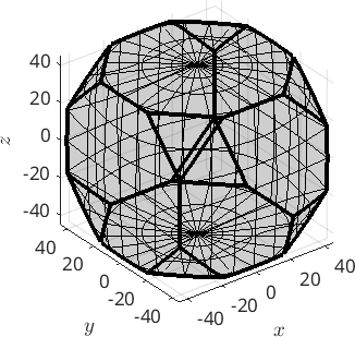

hold on
plot(ori,ind2color(c))
caxis([1,5])
plot(center,'MarkerSize',10,'MarkerFaceColor','k','MarkerEdgeColor','k')
plot(centerRec,'MarkerSize',10,'MarkerFaceColor','r','MarkerEdgeColor','k')
hold off

plot 2000 random orientations out of 3000 given orientations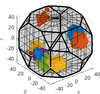

%check the accuracy of the recomputed centers
min(angle_outer(center,centerRec)./degree)

ans =
    0.3032    0.3298    0.2366    0.5450    0.1580

odfRec = calcDensity(ori)
[~,centerRec2] = max(odfRec,'numLocal',5)
min(angle_outer(center,centerRec2)./degree)

odfRec = SO3FunHarmonic (m3̅m → y↓→x)
  bandwidth: 25
  weight: 1
 
 
centerRec2 = orientation (m3̅m → y↓→x)
  size: 5 x 1
 
  Bunge Euler angles in degree
     phi1     Phi    phi2
  195.003 36.0515 142.611
  352.005 38.0716 13.7149
  302.885 43.5636 69.7739
  228.219  48.963 116.827
  146.085 24.0748 190.044
 
ans =
    0.4582    0.6089    0.1909    0.8792    0.6571

Citing this page. This page is part of the documentation of MTEX, a free and open source MATLAB toolbox for analyzing and modeling crystallographic textures. It was written by The MTEX Developers and is published at https://mtex-toolbox.github.io/orientation.doHClustering.html. If you use MTEX, or reuse text or figures from this page, in your research, please cite

F. Bachmann, R. Hielscher, H. Schaeben: Texture Analysis with MTEX - Free and Open Source Software Toolbox, Solid State Phenomena 160 (2010), 63-68. 10.4028/www.scientific.net/SSP.160.63

BibTeX

@article{bachmann2010mtex,
  author  = {F. Bachmann and R. Hielscher and H. Schaeben},
  title   = {Texture Analysis with MTEX - Free and Open Source Software Toolbox},
  journal = {Solid State Phenomena},
  volume  = {160},
  pages   = {63-68},
  year    = {2010},
  doi     = {10.4028/www.scientific.net/SSP.160.63},
  url     = {https://doi.org/10.4028/www.scientific.net/SSP.160.63}
}

Other papers describing specific MTEX methods are listed under Publications — please cite the one that best fits your application. The MTEX source code is licensed under the GNU General Public License v2.0; the text and figures of this documentation are licensed under CC BY 4.0, which permits reuse — including by automated systems — provided The MTEX Developers and this page are credited.