Sigle Slip Model

Details to this model can be found in

The Continuity Equation

The evolution of the orientation distribution function (ODF) \(f(g)\) with respect to a crystallographic spin \(\Omega(g)\) is governed by the continuity equation

\[\frac{\partial}{\partial t} f + \nabla f \cdot \Omega + f \text{ div } \Omega = 0\]

The solution of this equation depends on the initial texture \(f_0(g)\) at time zero and the crystallographic spin \(\Omega(g)\). In this model we assume the initial texture to be isotropic, i.e., \(f_0 = 1\) and the crystallographic spin be associated with a single slip system. The full ODF will be later modeled as a superposition of the single slip models.

In this example we consider Olivine with has orthorhombic symmetry

csOli = crystalSymmetry('222',[4.779 10.277 5.995],'mineral','olivine');
csOrtho = crystalSymmetry('222',[18.384, 8.878, 5.226],'mineral','orthopyroxene');

and the basic slip systems in olivine and orthopyroxene

sSOli = slipSystem(Miller({1,0,0},{1,0,0},{0,0,1},csOli,'uvw'),...
  Miller({0,1,0},{0,0,1},{0,1,0},csOli,'hkl'))

sSOrtho = slipSystem(Miller({0,0,1},csOrtho,'uvw'),...
  Miller({1,0,0},csOrtho,'hkl'))

sSOli = slipSystem (olivine)
 size: 1 x 3
 
  u    v    w  | h    k    l CRSS
  1    0    0    0    1    0    1
  1    0    0    0    0    1    1
  0    0    1    0    1    0    1
 
sSOrtho = slipSystem (orthopyroxene)
 
  u    v    w  | h    k    l CRSS
  0    0    1    1    0    0    1

To each of the slip systems we can associate an orientation dependent Schmid or deformation tensor \(S(g)\)

S = sSOli.deformationTensor

S = tensor (olivine)
  size: 1 x 3    
  rank: 2 (3 x 3)

and make for the orientation dependent strain rate tensor \(e(g)\) the ansatz \(e_{ij}(g) = \gamma(g) S_{ij}(g)\). Fitting this ansatz to a given a macroscopic strain tensor

E = 0.3 * strainRateTensor([1 0 0; 0 0 0; 0 0 -1])

E = strainRateTensor (xyz)
  rank: 2 (3 x 3)
 
 *10^-2
  30   0   0
   0   0   0
   0   0 -30

via minimizing the square difference

\[\int_{SO(3)} \sum_{i,j} (e_{i,j}(g) - E_{i,j})^2 dg \to \text{min}\]

the orientation dependent strain rate tensor is identified as

\[e(g) = 2 \left< S(g), E \right> S(g)\]

and the corresponding crystallographic spin tensor as

\[\Omega_i(g) = \epsilon_{ijk} e_{jk}(g)\]

This can be modeled in MTEX via

% this is in crystal coordinates
% Omega = @(ori) SO3TangentVector(spinTensor(((ori * S(2)) : E) .* S(2)));
% Omega = @(ori) 0.5 * EinsteinSum(tensor.leviCivita,[1 -1 -2],(ori * S(1) : E) .* (S(2)),[-1 -2])

% this is in specimen coordinates
Omega = @(ori) -SO3TangentVector(spinTensor(((ori * S(2)) : E) .* (ori * S(2))));

% turn in into a harmonic function
Omega = SO3VectorFieldHarmonic.quadrature(Omega,csOli)

Omega = SO3VectorFieldHarmonic (olivine → xyz)
  bandwidth: 3
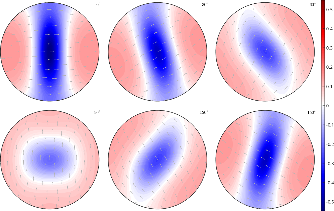
  tangent space: leftVector

% We may visualize the orientation dependence of the spin tensor by plotting
% its divergence in sigma sections and on top of it the spin tensors as a
% quiver plot

plotSection(div(Omega),'sigma','noGrid')
mtexColorMap blue2red
mtexColorbar

hold on
plot(Omega,'add2all','linewidth',1,'color','k')
hold off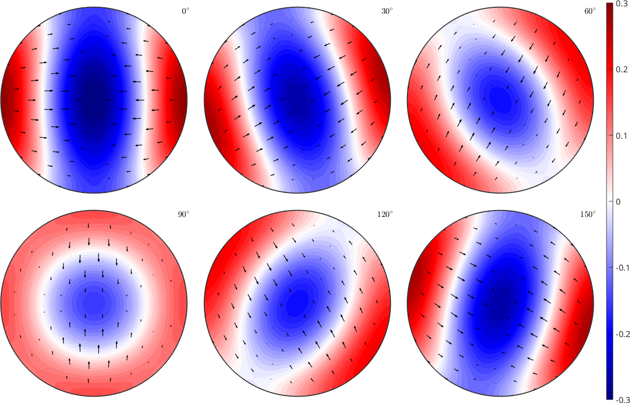

The divergence plots can be read as follows. Negative (blue) regions indicate orientations that increase in volume, whereas positive regions indicate orientations that decrease in volume. Accordingly, we expect the texture to become more and more concentrated within the blue regions. In the example example illustrated above with only the second slip system being active, we would expect the c-axis to align more and more with the the z-direction.

Solutions of the Continuity Equation

The solutions of the continuity equation can be analytically computed and are available via the command SO3FunSBF. This command takes as input the specific slips system sS and the macroscopic strain tensor E

odf1 = SO3FunSBF(sSOli(1),E)
odf2 = SO3FunSBF(sSOli(2),E)
odf3 = SO3FunSBF(sSOli(3),E)
odf4 = SO3FunSBF(sSOrtho,E)

odf1 = SO3FunSBF (olivine → xyz)
 
    slip system: (010)[100]
    strain:      0.3 0 -0.3
 
odf2 = SO3FunSBF (olivine → xyz)
 
    slip system: (001)[100]
    strain:      0.3 0 -0.3
 
odf3 = SO3FunSBF (olivine → xyz)
 
    slip system: (010)[001]
    strain:      0.3 0 -0.3
 
odf4 = SO3FunSBF (orthopyroxene → xyz)
 
    slip system: (100)[001]
    strain:      0.3 0 -0.3

Lets check our expectation from the last paragraph by visualizing the odf corresponding to the second slip system in sigma sections

figure(1)
plotSection(odf2,'sigma')
mtexColorbar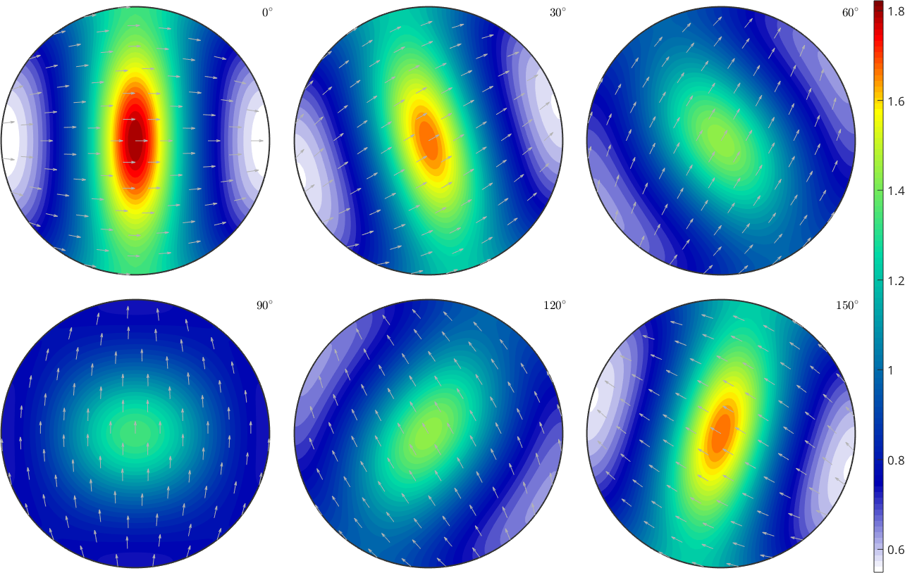

We observe exactly the concentration of the c-axis around z as predicted by the model. This can be seen even more clear when looking a the pole figures

h = Miller({1,0,0},{0,1,0},{0,0,1},csOli);

plotPDF(odf2,h,'resolution',2*degree,'colorRange','equal')
mtexColorbar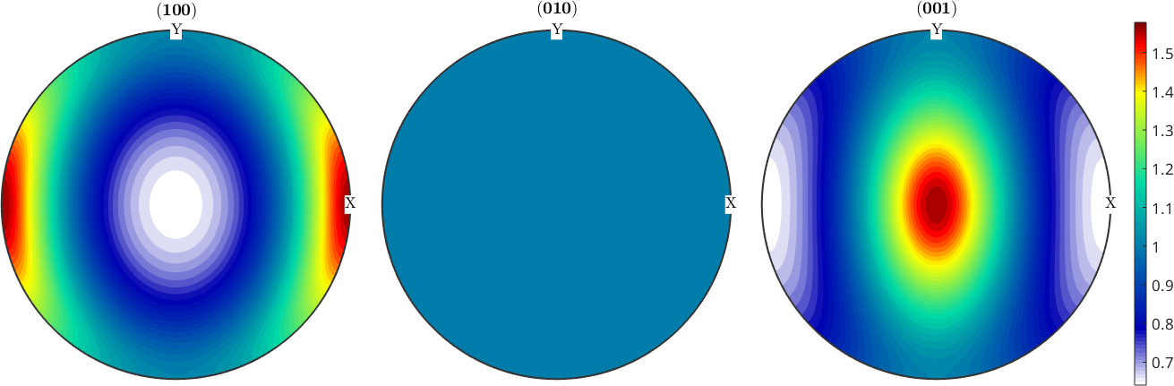

We could also have computed the solution of the continuity equation numerically. To this end we utilize the command doEulerStep which takes as input the crystallographic spin tensor Omega, the initial odf odf0 and the number of iterations to be performed.

% the starting ODF
odf0 = uniformODF(csOli);

% the transformed ODF
odf = doEulerStep(2*Omega,odf0,40)

figure(2)
plot(odf,'sigma')
mtexColorbar

odf = SO3FunHarmonic (olivine → xyz)
  bandwidth: 28
  weight: 1

Indeed the error between the numerical solution and the theoretical solution is neglectable small. We may quantify the difference by

mean(abs(odf - odf2))

ans =
    0.0011

For completeness the pole figures of the other two basis functions.

plotPDF(odf1,h,'resolution',2*degree,'colorRange','equal')
mtexColorbar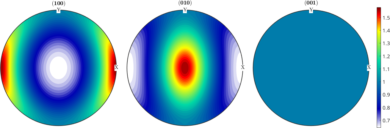

plotPDF(odf3,h,'resolution',2*degree,'colorRange','equal')
mtexColorbar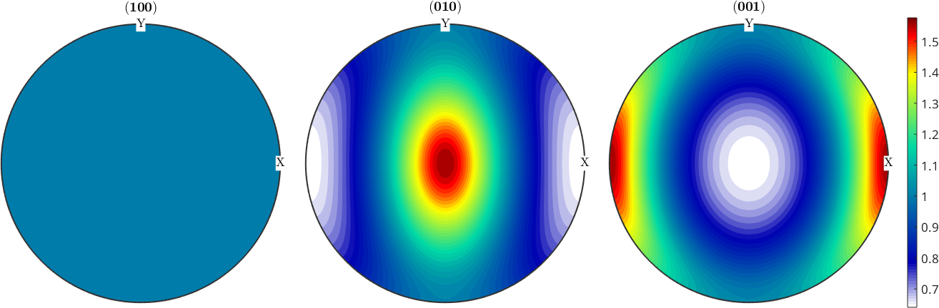

We observe that the pole figure with respect to \(n \times b\) is always uniform, where \(n\) is the slip normal and \(b\) is the slip direction.

Since in practice all three slip systems are active we can model the resulting ODF as a linear combination of the different basis functions

plotPDF(odf1 + odf2 + odf3,h,'resolution',2*degree,'colorRange','equal')
mtexColorbar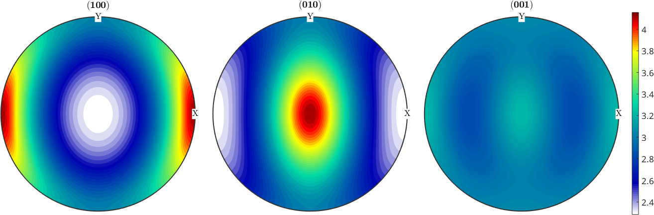

Checking the for steady state

We may also check for which orientations an ODF is already in a steady state of the continuity equation, i.e., the time derivative \(\text{div}(f \Omega) = 0\) is zero.

plotSection(div(odf2 .* Omega),'sigma')
mtexColorMap blue2red
mtexColorbar
setColorRange(max(abs(clim))*[-1,1])