On this page, we want to cover the topic of function approximation from discrete values on the sphere. To simulate this, we have stored some nodes and corresponding function values which we can load. The csv-file contains the \(x\)-, \(y\)-, and \(z\)-component of the nodes and the function value in the fourth column. Lets import these data using the function load
fname = fullfile(mtexDataPath, 'vector3d', 'smiley.csv');
[nodes, S] = vector3d.load(fname,'columnNames',{'x','y','z','values'});
The second output S is a struct that contains a field S.values with the function values from the fourth column. Next, we can make a scatter plot to see, what we are dealing with
scatter(nodes, S.values, 'upper');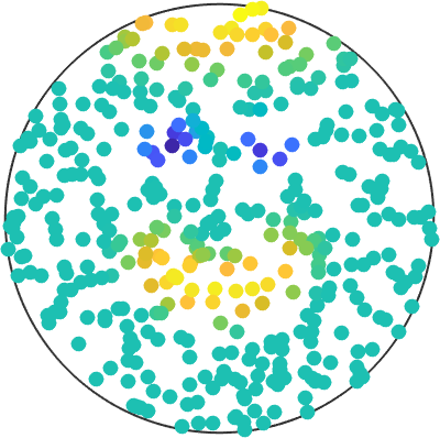
Now, we want to find a function which coincides with the given function values in the nodes reasonably well.
Interpolation
The idea of the first approach is fairly simple. We create a function which has exactly the value of the given data in the nodes. But we still have to decide what happens inbetween these nodes. For that, we linearly interpolate between them, similarly as Matlab plots a one-dimensional function
close all
plot(rand(10,1), '-s','linewidth',2)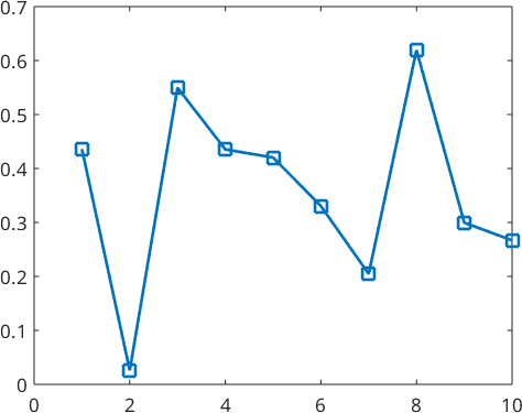
With some mathematics we can lift this concept to the sphere. This is done by the interp command of the class vector3d when the argument 'linear' is given
sFTri = interp(nodes, S.values, 'linear');To see that we really have the exact function values, we can evaluate sFTri of type S2FunTri and compare it with the original data values.
norm(eval(sFTri, nodes) - S.values)ans =
2.0347e-14Indeed, the error is within machine precision. Now we can work with the function defined on the whole sphere. We can, for instance, plot it
contourf(sFTri, 'upper');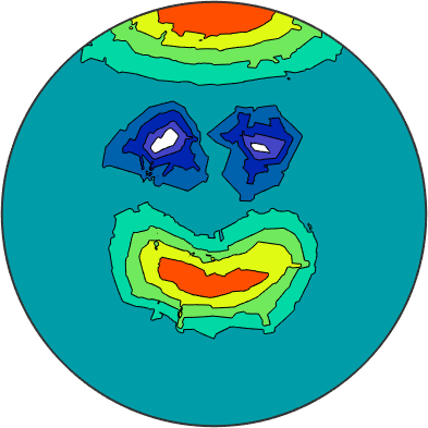
That does not look like the happy smiley face we had in mind. There are other variants to fill the gaps between the data nodes, still preserving the interpolation property, which may improve the result. But if we don't restrict ourselves to the given function values in the nodes, we have more freedom, which can be seen in the case of approximation.
Approximation
In contrast to interpolation we are now not restricted to the function values in the nodes but still want to keep the error reasonably small. One way to achieve this is to approximate it with a series of spherical harmonics. We don't take as many spherical harmonics as there are nodes, such that we are in the overdetermined case. In that way we don't have a chance of getting the error in the nodes zero but hope for a smoother approximation. This can be achieved by the interp command of the class vector3d when the argument 'harmonic'
sF = interp(nodes, S.values, 'harmonic');
contourf(sF, 'upper');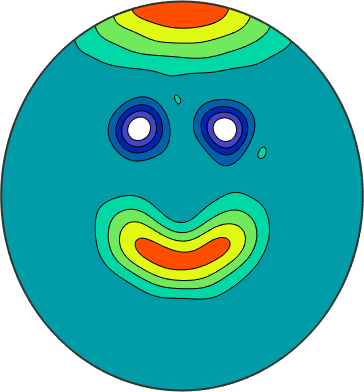
Plotting this function, we can immediately see, that we have a much smoother function. But one has to keep in mind that the error in the data nodes is not zero as in the case of interpolation.
norm(eval(sF, nodes) - S.values)ans =
0.0606But this may not be of great importance like in the case of function approximation from noisy function values, where we don't know the exact function values anyways.
The strategy underlying the interp(...,'harmonicApproximation')-command to obtain such an approximation works via spherical harmonics (Basics of spherical harmonics). For that, we seek for so-called Fourier-coefficients \({\bf \hat f} = (\hat f_0^0,\dots,\hat f_M^M)^T\) such that
\[ g(x) = \sum_{m=0}^M\sum_{l = -m}^m \hat f_m^l Y_m^l(x) \]
approximates our function. A basic strategy to achieve this is through least squares, where we minimize the functional
\[ \sum_{n=1}^N|f(x_n)-g(x_n)|^2 \]
for the data nodes \(x_n\), \(n=1,\dots,N\), \(f(x_n)\) the target function values and \(g(x_n)\) our approximation evaluated in the given data nodes.
This can be done by the lsqr function of Matlab, which efficiently seeks for roots of the derivative of the given functional (also known as normal equation). In the process we compute the matrix-vector product with the Fourier-matrix multiple times, where the Fourier-matrix is given by
\[ F = [Y_m^l(x_n)]_{n = 1,\dots,N;m = 0,\dots,M,l = -m,\dots,m}. \]
This matrix-vector product can be computed efficiently with the use of the nonequispaced spherical Fourier transform NFSFT.
We end up with the Fourier-coefficients of our approximation \(g\), which describe our approximation.