
An orientation grid is a finite set of nodes in orientation space. Such grids are used to evaluate or approximate an ODF, to search for a best fit, and to provide orientations to another numerical method.
Read Orientations and Fundamental Regions first. The spherical counterpart is Spherical Grids.
The nodes should usually be spread uniformly with respect to volume on \(\mathrm{SO}(3)\), not with respect to the coordinates used to describe a rotation. No finite construction is perfectly uniform, and different grids preserve different useful structures.
For these figures, the plotting convention lays out the specimen reference frame with y up and x to the right. It does not alter the grid.
plottingConvention.default('y↑→x');

% cubic crystal symmetry and trivial specimen symmetry
cs = crystalSymmetry('432');
The Equispaced Grid
equispacedSO3Grid covers the fundamental region of the supplied crystal and specimen symmetries with nearly constant node spacing. Here the specimen symmetry is the trivial default. Both global constructors accept a second symmetry. For an orientation it is a specimen symmetry; for a misorientation it is the crystal symmetry on the other side.
The 'resolution' is a target spacing. The construction adjusts the angular steps to fit the fundamental region, so it is not a promise that every pair of neighbouring nodes is exactly \(5^\circ\) apart.
equiGrid = equispacedSO3Grid(cs,'resolution',5*degree)equiGrid = SO3Grid (432 → y↑→x)
grid: 4923 orientations, resolution: 5°The summary reports 4923 orientations and identifies the result as an SO3Grid with \(5^\circ\) resolution. An axis--angle plot shows the nodes throughout the cubic fundamental region.
plot(equiGrid,'axisAngle','all','MarkerSize',2);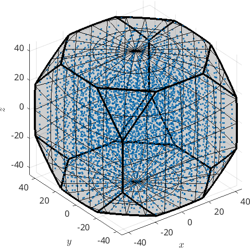
The point cloud has no large empty patch or concentrated band. Its visual density still changes under axis--angle coordinates, so this plot alone cannot establish equal volume in orientation space.
The Regular Euler Grid
regularSO3Grid instead takes regular steps in the three Euler angles. The same nominal resolution creates many more nodes.
regularGrid = regularSO3Grid(cs,'resolution',5*degree);

gridCounts = [length(equiGrid),length(regularGrid)]
gridCounts =
4923 24624The two entries are 4923 and 24624. Thus the regular grid has five times as many orientations at the same nominal resolution.
plot(regularGrid,'axisAngle','all','MarkerSize',1);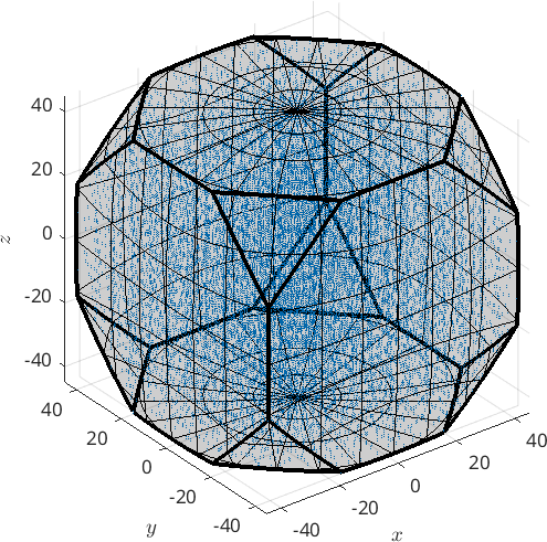
Lines and dense bands remain visible after transformation from Euler angles to axis--angle coordinates. They are the signature of regular coordinate steps, not extra resolution distributed uniformly over orientation space.
Why Regular Euler Steps Are Not Uniform
In Bunge Euler angles, the invariant volume element on rotation space is proportional to
\[ \sin\Phi\,\mathrm{d}\varphi_1\,\mathrm{d}\Phi\,\mathrm{d}\varphi_2. \]
Equal increments of \(\Phi\) therefore represent unequal volumes. A regular Euler grid places too many equal-weight nodes where the coordinate map is compressed. This is the three-dimensional counterpart of longitude lines meeting at the poles of a spherical grid.
The Fibonacci Grid
fibonacciSO3Grid places its nodes along a spiral through orientation space. There are no coordinate steps to be rounded, so the number of nodes is a free parameter.
fibGrid = fibonacciSO3Grid(cs,'resolution',5*degree);

fibCounts = [length(fibGrid),length(fibonacciSO3Grid(cs,'points',5000))]
fibCounts =
4994 5034The two entries are 4994 and 5034, so the spiral meets a requested node count to within one percent. It is the construction to reach for when a fixed budget of orientations is the constraint.
plot(fibGrid,'axisAngle','all','MarkerSize',2);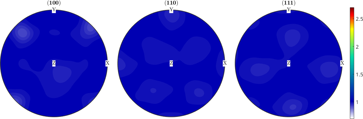
The spiral is generated over all of \(\mathrm{SO}(3)\) and then restricted to the fundamental region, so the nodes fill the same region as the equispaced grid. They carry no bands and no shell structure.
An Equal-Weight Uniformity Diagnostic
A practical diagnostic treats every node as the centre of an equally weighted kernel. If the nodes represent the invariant volume uniformly, the resulting ODF should be close to the uniform value 1. Its pole figures should therefore also be nearly flat at 1.
The result depends on the kernel halfwidth, which is made explicit here. It tests equal-weight node placement at that smoothing scale. It does not prove equidistribution, measure nearest-neighbour spacing, or turn the nodes into a quadrature rule.
h = Miller({1,0,0},{1,1,0},{1,1,1},cs);
equiOdf = unimodalODF(equiGrid,'halfwidth',10*degree);

plotPDF(equiOdf,h);
setColorRange([0.7 2.7]);
mtexColorbar;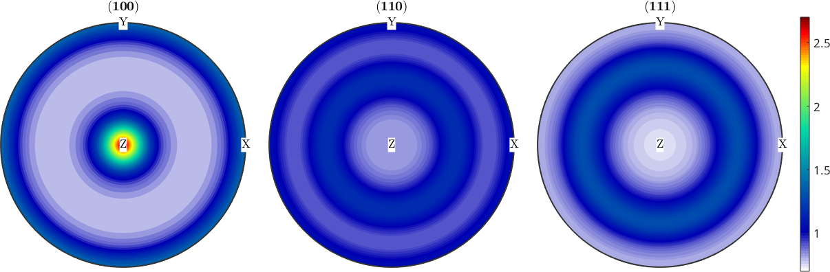
On the common colour range used for both constructions, all three pole figures appear flat. Their values span 0.93 to 1.02, so the equispaced grid stays within about 7 percent of 1 in this diagnostic. Flat to within a few percent is what a usable grid looks like.
regularOdf = unimodalODF(regularGrid,'halfwidth',10*degree);

plotPDF(regularOdf,h);
setColorRange([0.7 2.7]);
mtexColorbar;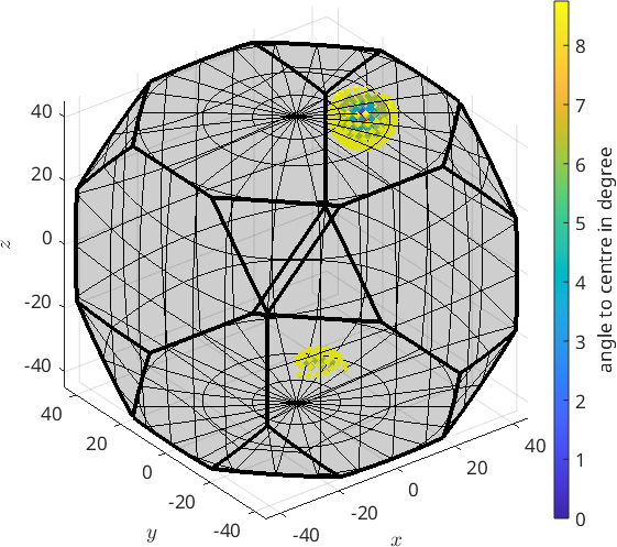
The regular grid develops a strong peak. Its (100) pole figure spans 0.79 to 2.62, and the three pole figures together span 0.75 to 2.62. The extra points therefore do not buy equal-weight uniformity.
fibOdf = unimodalODF(fibGrid,'halfwidth',10*degree);

plotPDF(fibOdf,h);
setColorRange([0.7 2.7]);
mtexColorbar;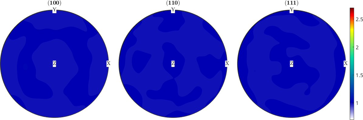
The Fibonacci grid spans 0.99 to 1.02, within about 2 percent of 1, at the same node count as the equispaced grid.
Choosing a Global Grid
Use a regular grid when values must lie on an Euler-angle raster, for example when exporting an ODF to a format that expects one. Use an equispaced grid when approximately uniform equal-weight nodes matter more than rectangular Euler indexing.
A nearly uniform point set is not automatically an integration rule. Exactness for a class of band-limited functions requires nodes together with their prescribed weights; see Quadrature of Rotational Functions.
Grids Around a Given Orientation
localOrientationGrid covers a ball around one orientation rather than the full symmetry-reduced region. This is the useful construction for a local search or a perturbation study.
center = orientation.byEuler(10*degree,20*degree,30*degree,cs);
localGrid = localOrientationGrid(center,10*degree, ...
  'resolution',2.5*degree);

localCount = length(localGrid)
maxLocalAngle = max(angle(localGrid,center)) ./ degree
localCount =
265
maxLocalAngle =
8.7500The grid contains 265 orientations arranged in shells about the centre. Its outermost shell is \(8.75^\circ\) from the centre, half a resolution step inside the requested \(10^\circ\) radius.
plot(localGrid,angle(localGrid,center)./degree, ...
  'axisAngle','all','MarkerSize',4);
hold on
plot(center,'MarkerFaceColor','r','MarkerSize',10);
hold off
mtexColorbar('title','angle to centre in degree');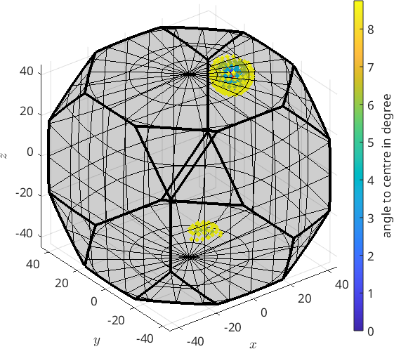
The red point marks the centre, and colour records rotational distance from it. The ball appears as two patches because it crosses a boundary of the fundamental region and wraps to a symmetrically equivalent face. Despite that split in the plot, every node lies within the requested ball.
Further Reading
- H.-J. Bunge, Texture Analysis in Materials Science: Mathematical Methods, Butterworths, 1982. Sections on the invariant measure and Euler space give the texture-analysis foundation for the volume element above.
- A. Morawiec, Orientations and Rotations: Computations in Crystallographic Textures, Springer, 2004. This book develops rotation-space geometry and symmetry-reduced regions.
- A. Yershova, S. Jain, S. M. LaValle and J. C. Mitchell, Generating Uniform Incremental Grids on SO(3) Using the Hopf Fibration, The International Journal of Robotics Research 29(7), 801--812, 2010. The paper compares criteria for uniform deterministic grids on rotation space.
- D. Roşca, A. Morawiec and M. De Graef, A New Method of Constructing a Grid in the Space of 3D Rotations and Its Applications to Texture Analysis, Modelling and Simulation in Materials Science and Engineering 22, 075013, 2014. This paper develops a volume-preserving cubochoric construction for texture analysis.
- M. Alexa, Super-Fibonacci Spirals: Fast, Low-Discrepancy Sampling of SO(3), Proceedings of the IEEE/CVF Conference on Computer Vision and Pattern Recognition, 8291--8300, 2022. This paper gives the spiral construction behind
fibonacciSO3Gridand the two irrational ratios it uses.
Next
Curves through orientation space, along which many real textures lie, are Fibres of Orientations. Sampling an ODF statistically rather than placing a grid is Random Sampling.
Citing this page.
This page is part of the documentation of
MTEX, a free and open
source MATLAB toolbox for analyzing and modeling crystallographic textures.
It was written by The MTEX Developers and is published at
https://mtex-toolbox.github.io/OrientationGrid.html.
If you use MTEX, or reuse text or figures from this page, in your research,
please cite
F. Bachmann, R. Hielscher, H. Schaeben: Texture Analysis with MTEX - Free and Open Source Software Toolbox, Solid State Phenomena 160 (2010), 63-68. 10.4028/www.scientific.net/SSP.160.63
BibTeX
@article{bachmann2010mtex,
  author  = {F. Bachmann and R. Hielscher and H. Schaeben},
  title   = {Texture Analysis with MTEX - Free and Open Source Software Toolbox},
  journal = {Solid State Phenomena},
  volume  = {160},
  pages   = {63-68},
  year    = {2010},
  doi     = {10.4028/www.scientific.net/SSP.160.63},
  url     = {https://doi.org/10.4028/www.scientific.net/SSP.160.63}
}
Other papers describing specific MTEX methods are listed under Publications — please cite the one that best fits your application. The MTEX source code is licensed under the GNU General Public License v2.0; the text and figures of this documentation are licensed under CC BY 4.0, which permits reuse — including by automated systems — provided The MTEX Developers and this page are credited.