Grains as three dimensional objects are stored in MTEX as variables of type grain3d. Basic properties and operations are described in the sections Properties of Three-Dimensional Grains and Operations with Three-Dimensional Grains.
In this section we discuss how to import three dimensional grains from Dream3d and Neper.
Import Grains from Dream3d
In order to import grain data we use the command grain3d.load
% specify the file name
fname = fullfile(mtexDataPath,'EBSD','SmallIN100_MeshStats.dream3d');
grains = grain3d.load(fname);

% for triangulated data sets it may be useful to plot them without lines
plot(grains,grains.meanOrientation,'LineStyle','none','micronbar','off')

% use a nice plotting convention
how2plot = plottingConvention.default3D;
setCamera(how2plot)
Warning: Grains imported from Dream3d may not have set there normals
consistently. Please run <a href="matlab:grains=grains.orientFaces">grains=grains.orientFaces</a>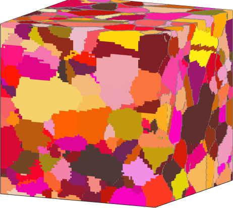
Unfortunately, the boundary face normals provided by Dream3d sometimes come with no orientation. In this case we have MTEX to compute the orientation of the faces using the command orientFaces. This may take some time and requires the free and open source GPTToolbox https://de.mathworks.com/matlabcentral/fileexchange/49692-gptoolbox> to be installed.
grains = grains.orientFacesgrains = grain3d
Phase Grains Volume Mineral Symmetry Crystal reference frame
2 794 15625 unknown 622 X||a*, Y||b, Z||c*
boundary faces: 757564
Properties: meanRotationSimilarly as with two dimensional grains we can select individual grains by arbitrary constraints. For instance we can find the largest grain by
% index of the grain with the largest volume
[~,id] = max(grains.volume)

plot(grains(id),'edgeAlpha',0.15,'micronBar','off')
setCamera(how2plot)
id =
623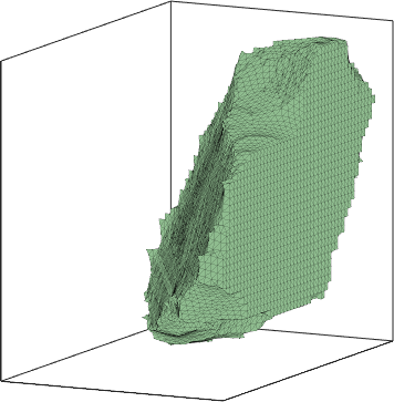
Slicing the 3d grains by a plane using the command slice results in 2d grains comparable to what can be reconstructed from 2d EBSD maps.
% define the plane by a normal direction and a point
plane = plane3d(vector3d(1,1,1),vector3d(-20,20,-15));

% compute the sliced grains
grains2 = slice(grains,plane)

% plot them
plot(grains2,grains2.meanOrientation,'micronbar','off')

setCamera(how2plot)
grains2 = grain2d (y↑→x)
Phase Grains Pixels Mineral Symmetry Color
2 187 187 unknown 622
boundary segments: 7177 (655 µm)
inner boundary segments: 0 (0 µm)
triple points: 269
Properties: meanRotation, Id3d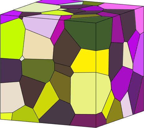
It might be reasonable to adjust the plotting convention such that the normal direction grains2.N points out of screen.
how2plot2 = plottingConvention;
how2plot2.outOfScreen = grains2.N;
how2plot2.east = vector3d(1,-1,0);

setCamera(how2plot2), axis off, xlabel('') , ylabel('')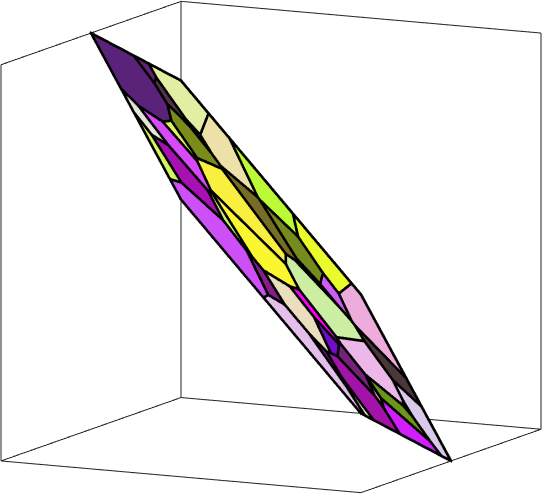
Import Grains from Neper
Neper is a software package for the simulation of three dimensional microstructures. After installation it can be directly called by MTEX. The general workflow is explained here. Here we use it to quickly generate a copper microstructure with specific texture and specific distribution of boundary normals.
% set up the communication with Neper
neper.init;
neper.geometry = "cube(2,2,1)";

% define a texture
cs = crystalSymmetry.load('quartz.cif','color','lightblue');
odf = fibreODF(cs.cAxis,vector3d(1,1,1));

numGrains = 300;
grains = neper.simulateGrains(numGrains,odf,'silent')
% or you can load an existing tessellation file
%grains = grain3d.load('allgrains.tess','CS',cs)
grains = grain3d
Phase Grains Volume Mineral Symmetry Crystal reference frame
2 300 4 Quartz 321 X||a*, Y||b, Z||c*
boundary faces: 2032
Properties: meanRotation% colorize by mean orientation
plot(grains,grains.meanOrientation,'micronbar','off','faceAlpha',0.5)
setCamera(how2plot)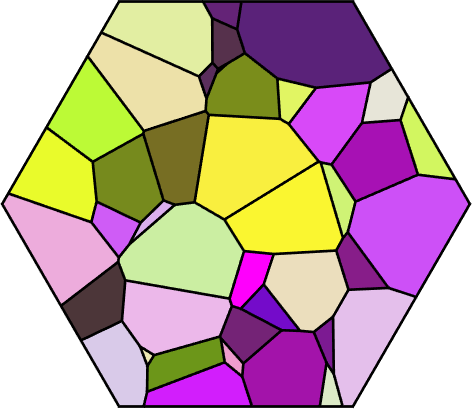
Slicing
Let us slice this 3d data set as well
% make all slices passing through the center point of the cube
P0 = vector3d(0.5,0.5,0.5);

% with normal (0,0,1)
N = vector3d(0,0,1);

grains_2d = grains.slice(N,P0)

plot(grains_2d,grains_2d.meanOrientation,'micronbar','off','linewidth',3)
setCamera(how2plot)
grains_2d = grain2d (y↑→x)
Phase Grains Pixels Mineral Symmetry Color
2 99 99 Quartz 321
boundary segments: 298 (41 µm)
inner boundary segments: 0 (0 µm)
triple points: 165
Properties: meanRotation, Id3d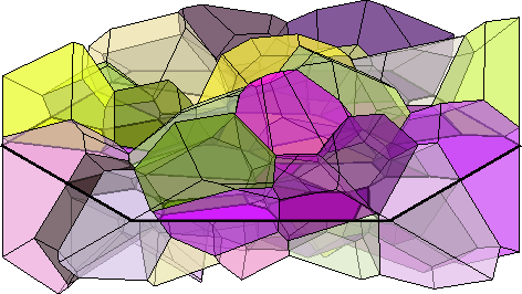
Grains intersecting a slice
Using the function intersected we can identify all grains that intersect a given plane. Lets simply add 3d the shapes of all grains intersecting the plane.
isInter = grains.intersected(N,P0);

hold on
plot(grains(isInter),grains(isInter).meanOrientation,'faceAlpha',0.6,'linewidth',0.5)

%[a,b,c] = grains(isInter).principalComponents;
%plotEllipsoid(grains(isInter).centroid,a,b,c,'faceAlpha',0.5)
hold off

%setCamera(plottingConvention.default3D)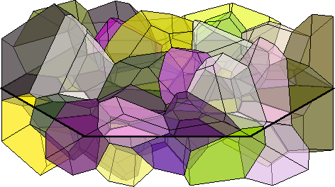
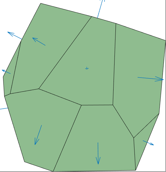
Plot the normal directions of a single grain
The following code shows how to visualize the face normals
grains = grains(1)

% multiplication with I_GF flips the boundary normals to point out of the
% grain
dir = full(grains.I_GF(1,:)).' .* grains.boundary.N

plot(grains)
hold on
quiver(grains.boundary,dir)
hold off
grains = grain3d
Phase Grains Volume Mineral Symmetry Crystal reference frame
2 1 0.0084 Quartz 321 X||a*, Y||b, Z||c*
boundary faces: 11
Id Phase Pixels meanRotation
1 2 1 (323.6°,125.7°,281.9°)
dir = vector3d (y↑→x)
size: 11 x 1
x y z
0 0 -1
0.273 0.962 -0.0279
0.896 -0.0808 0.437
-0.883 0.45 -0.133
0.886 -0.365 0.286
-0.557 0.33 0.762
0.0112 -0.109 0.994
0.0119 -0.825 0.564
-0.259 -0.759 0.598
-0.725 0.322 0.609
-0.98 -0.145 -0.136