Convex Hull Based Shape Parameters

Stretch a rubber band around a grain and let it snap tight: what you get is the convex hull. A convex grain is its own hull, however large or elongated it is. A bay or inlet leaves a gap between the grain and its hull, so comparing the two isolates lobateness: departure from a convex outline.

This page assumes the direct measurements introduced in Shape Parameters. The shapes below are artificial, chosen so that each measure has something to react to.

% import the artificial grain shapes
plottingConvention.default('y↑→x');
mtexdata testgrains silent

% select and smooth a few interesting grains
grains = smoothBoundary(grains('id',[2 3 9 11 15 16 18 23 31 33 38 40]),3);

Boundary smoothing is not optional here. On an unsmoothed square grid every boundary segment is horizontal or vertical. The perimeter then measures the cityblock distance and comes out too long, while the convex hull cuts the corners. The difference between the two would be dominated by the grid. For very small grains even smoothing does not save it, and the numbers below should not be trusted.

hull returns the hulls as grains, so everything that works on grains works on them.

% compute convex hull grains
chGrains = grains.hull;

% plot the original grains
plot(grains,'micronbar','off'), legend off

% and on top of them the convex hull
hold on
plot(chGrains.boundary,'lineWidth',2,'lineColor','r')
text(grains,arrayfun(@num2str,grains.id,'UniformOutput',false))
hold off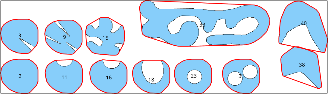

Where a grain is convex the red line follows its outline; where it is indented the line cuts across. The labels are grain ids used in the table below. Hulls may overlap even when the grains do not. A hull outline no longer separates two grains. The second phase of every hull boundary segment is therefore set to 'notIndexed'.

Four ways to measure an indentation

The relative difference between the perimeter of the grain and that of its hull reacts most strongly to thin, narrow indentations - a crack that does not quite cut the grain in two adds a great deal of perimeter and almost no area. The result, deltaP, is a dimensionless percentage.

deltaP = 100 * (grains.perimeter-chGrains.perimeter) ./ grains.perimeter;

paris, the Percentile Average Relative Indented Surface, compares the same two perimeters relative to the hull and doubles that ratio. It is the conventional name in the literature, and grains.paris computes it directly.

paris = 200 * (grains.perimeter - chGrains.perimeter) ./ chGrains.perimeter;

Comparing the areas instead of the perimeters reacts to broad, shallow lobes - a big bite out of a grain, which changes the area a lot and the perimeter hardly at all. The result, deltaA, is 100 times one minus the quantity often called solidity, the grain area divided by its hull area.

deltaA = 100 * (chGrains.area - grains.area) ./ chGrains.area;

Since the two react to different kinds of indentation, combining them gives radiusD, a measure that responds to both.

radiusD = sqrt(deltaP.^2 + deltaA.^2);

Compare the measures

The table makes the values behind the colour maps explicit. A zero in a perimeter-based column means that the outer outline is convex. deltaA is zero only when the grain fills its hull, with no hole. deltaP and deltaA are below 100, whereas paris has no upper bound despite being reported as a percentage.

indentationSummary = table(grains.id,grains.hasHole,deltaP,grains.paris,...
  deltaA,radiusD,'VariableNames',...
  {'grainId','hasHole','deltaP','paris','deltaA','radiusD'})

indentationSummary =
  12×6 table
    grainId    hasHole    deltaP    paris     deltaA     radiusD
    _______    _______    ______    ______    _______    _______
       2        false     1.5993    3.2506    0.94143    1.8558 
       3        false     22.441    57.867     5.2569    23.048 
       9        false     45.108    164.35     8.6773    45.935 
      11        false     6.3239    13.502     8.4411    10.547 
      15        false     35.089    108.11     23.228     42.08 
      16        false     8.1283    17.695     11.266    13.892 
      18        false     27.222    74.809     41.946    50.005 
      23        true      1.5738     3.198     16.206    16.282 
      31        true      1.6069    3.2663     31.506    31.547 
      33        false       45.5    166.97     34.684    57.212 
      38        false     4.8281    10.146     16.891    17.567 
      40        false      14.32    33.426     31.414    34.524

Drawn side by side on the same shapes, the measures separate narrow from broad indentations:

plot(grains,deltaP,'layout',[2 2],'micronbar','off')
mtexTitle('deltaP')

nextAxis
plot(grains,grains.paris,'micronbar','off')
mtexTitle('paris')

nextAxis
plot(grains,deltaA,'micronbar','off')
mtexTitle('deltaA')

nextAxis
plot(grains,radiusD,'micronbar','off')
mtexTitle('radiusD')
mtexColorbar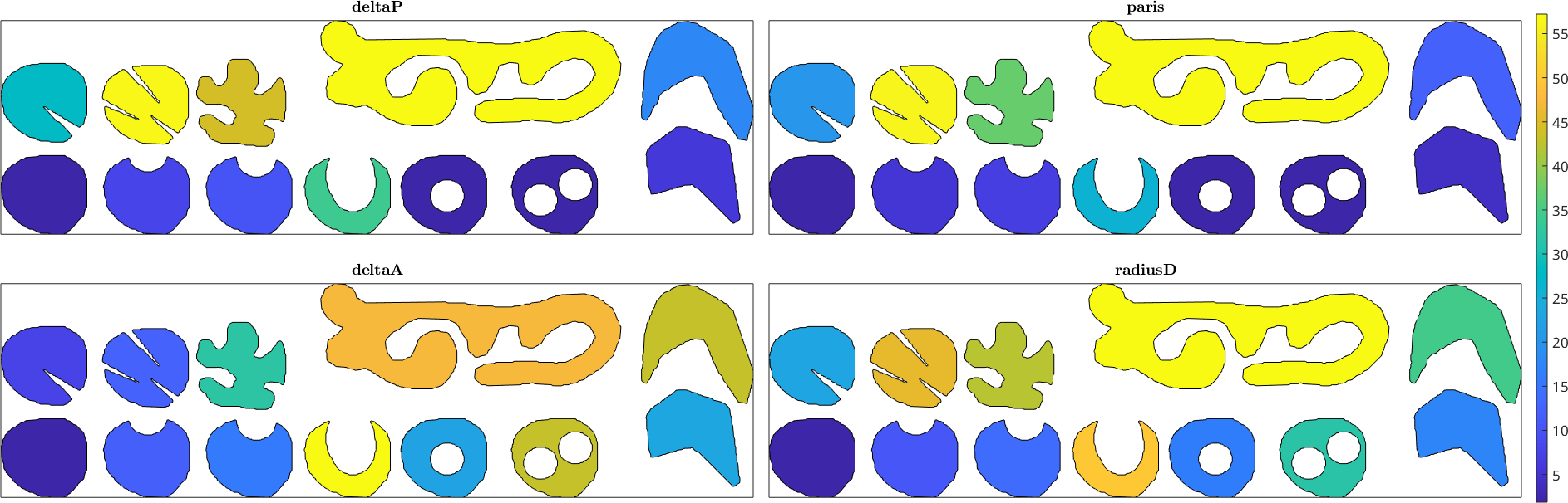

The first two maps rank the grains identically, as they must, being the same ratio written two ways - only the scale differs, paris running to 167 where deltaP stops at 46. The third map ranks them differently: the lobed grain scores 45 on deltaP against 9 on deltaA, all perimeter and almost no missing area, while the two discs with a hole score 1.6 on deltaP - as convex as the plain disc - and 16 and 32 on deltaA. radiusD puts both kinds high, which is what combining them is for.

The discs with holes are worth a second look, because they show what these measures are and are not counting. A hole and an inclusion are the same enclosure viewed from opposite sides. It is not an indentation of the outer outline, so the perimeter-based measures ignore it; paris explicitly removes inclusion loops before it measures. The area-based measure cannot ignore it, since the hull contains the hole and the grain does not. If a hole is not what you mean by lobateness, use deltaP or paris; if it is, use deltaA.

Which measure to report otherwise depends on the process being described. A dissolution front eats broad bays and shows up in deltaA; a partly healed fracture is a thin slot and shows up in deltaP.

These values also depend on pixel spacing and boundary smoothing. Use the same smoothBoundary settings for every map being compared, report them with the segmentation and resolution, and state the formula because other software uses names such as convexity and solidity for several different ratios.

References

Next

A convex hull discards every indentation. The Projection Parameters page instead keeps the width of each grain as a function of direction and develops shape-preferred orientation from those widths.

References

- Panozzo, R. and Hürlimann, H. (1983), A simple method for the quantitative discrimination of convex and convex-concave lines, Microscopica Acta 87, 169-176, introduced the PARIS factor.
- Heilbronner, R. and Keulen, N. (2006), Grain size and grain shape analysis of fault rocks, Tectonophysics 427, 199-216, developed the hull-area difference and applied both descriptors to fault rocks.
- Back, A. L., Kana Tepakbong, C., Bédard, L. P. and Barry, A. (2025), From rocks to pixels, Frontiers in Earth Science 13, reviews grain-shape descriptors and their inconsistent nomenclature across fields.