EBSD Simulation

A map-processing method is easiest to test on a map whose answer is known in advance. The simulateEBSD class constructs such a map one feature at a time. It can add orientation noise, a low-angle boundary, or an orientation gradient to a uniform field.

This makes it useful for checking denoising and KAM. It also supplies known input for GND and WBV calculations. Synthetic and experimental examples appear in Hielscher et al. (2019).

First read about orientations and misorientations. The page also assumes familiarity with grain reconstruction.

What is being simulated

simulateEBSD constructs an EBSD variable containing positions, a phase, and orientations. It does not generate diffraction patterns or model the detector, pattern indexing, spatial distortion, or failed measurements. A program such as EMsoft is needed for physics-based EBSD pattern simulation.

The class is designed for a single-grain orientation field. Use the Neper interface when polycrystal topology matters.

The object and its defaults

The object holds the map settings and the current simulated map. Its defaults specify coordinate limits of 100 by 100 and a unit step size. They do not create a map or add noise until the corresponding methods are called.

plottingConvention.default('y↓→x');

eS = simulateEBSD

eS = 
  simulateEBSD with properties:

          xdim: 100
          ydim: 100
      stepSize: 1
      domainID: []
      noiseFun: []
      noiseMax: 8.7266e-04
       EBSDsim: []
           axS: [1×1 vector3d]
       gradDir: [1×1 vector3d]
    mori_angle: 0.0017
          ori0: [1×1 orientation]
            CS: [1×1 crystalSymmetry]

A uniform orientation field

Set the coordinate limit, crystal symmetry, and reference orientation. The method makeMap then creates the EBSD variable in eS.EBSDsim.

eS.xdim = 200;
eS.CS = crystalSymmetry('mmm','Mineral','Kryptonite');
eS.ori0 = orientation.byEuler([0,pi/4,0]*degree,eS.CS);

eS.makeMap;
eS.EBSDsim

ipfKey = ipfColorKey(eS.CS);
plot(eS.EBSDsim,ipfKey.orientation2color(eS.EBSDsim.orientations));

ans = EBSD (y↓→x)
 
 Phase  Orientations     Mineral         Color  Symmetry  Crystal reference frame
     1  20000 (100%)  Kryptonite  LightSkyBlue       mmm                         
 
 Properties: emptyProp
 Scan unit : um
 X × Y × Z : [1 → 200] × [1 → 100] × [0 → 0]
 Normal vector: (0,0,1)

The summary reports 20,000 measurements of one indexed phase. The map has one colour because every measurement carries ori0 exactly. This is the known reference field to which the following features are added.

Adding orientation noise

Noise is a random rotation about a random axis in the specimen frame. noiseFun selects a uniform or lognormal distribution of rotation angles. For 'logn', the sampled angles are rescaled so that the largest equals noiseMax; noiseMax is not a parameter of a lognormal distribution.

eS.noiseFun = 'logn';
eS.noiseMax = 2*degree;
eS.addnoise;

noiseAngle = angle(eS.ori0,eS.EBSDsim.orientations)./degree;
fprintf(['Noise deviation: median %.2f degree; 90th percentile %.2f degree; ' ...
  'maximum %.2f degree\n'],median(noiseAngle),quantile(noiseAngle,0.9), ...
  max(noiseAngle));

plot(eS.EBSDsim,noiseAngle);
mtexColorbar('title','deviation from ori0 in degree');

Noise deviation: median 0.03 degree; 90th percentile 0.11 degree; maximum 2.00 degree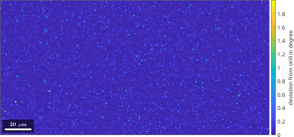

The deviation map shows many small rotations and a sparse long tail. Its printed maximum reaches the requested 2°. The median and 90th percentile describe the reproducible sample used here. This is orientation-level noise, not noise in simulated diffraction patterns.

A known low-angle boundary

A step feature is specified by a misorientation axis in the specimen frame and a total misorientation angle. addFeature_singleStep rotates one stepped domain relative to the other.

eS.axS = yvector;
eS.mori_angle = 3*degree;
eS.addFeature_singleStep;

Feature methods modify the orientations already in eS.EBSDsim. They therefore accumulate: this 3° step is added to the noisy map rather than to a fresh uniform map.

newMtexFigure('layout',[1,2]);

plot(eS.EBSDsim,angle(eS.ori0,eS.EBSDsim.orientations)./degree);
mtexTitle('deviation from ori0');

% classify the known step as an inner boundary
grains = eS.EBSDsim.calcGrains('angle',[10 1]*degree);
isStepSegment = xor(eS.domainID(grains.innerBoundary.ebsdId(:,1)), ...
  eS.domainID(grains.innerBoundary.ebsdId(:,2)));
stepBoundary = grains.innerBoundary(isStepSegment);
boundaryAngle = stepBoundary.misorientation.angle./degree;
fprintf(['Inner boundary: %d segments; mean %.2f degree; ' ...
  'range %.2f to %.2f degree\n'],length(boundaryAngle), ...
  mean(boundaryAngle),min(boundaryAngle),max(boundaryAngle));

nextAxis;
plot(grains);
hold on;
plot(stepBoundary,boundaryAngle,'linewidth',3);
hold off;
setColorRange([2.75 3.25]);
mtexColorbar('title','boundary angle in degree');

Inner boundary: 167 segments; mean 3.00 degree; range 2.88 to 3.23 degree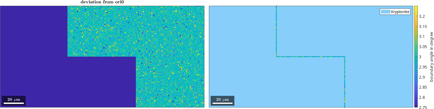

The left map contains one domain scattered around ori0 and another scattered around the 3° offset. The right map uses 10° as the grain-boundary threshold and 1° as the lower, subgrain threshold. The connected field is one grain. Its known step is stored in innerBoundary.

The narrow colour range makes variation along the boundary visible. The printed mean stays close to the imposed 3°. Its range records the noise that was added before the step. The count is the number of individual grain boundary segments along the stepped feature. Other short entries in innerBoundary can be caused by neighbouring noise rotations that differ by more than 1°. The domainID mask isolates the segments that cross the feature whose true location is known.

Synthetic noisy maps are particularly useful when the imposed boundary is close to the angular noise. See Germain et al. (2014).

Starting over with an orientation gradient

makeMap discards the accumulated features and restores a uniform field. For a gradient, gradDir gives the direction of increase in the specimen frame. Here mori_angle is the angle increment per spatial grid step, not the total angle used by the step feature.

eS.makeMap;
eS.axS = yvector;
eS.gradDir = xvector;
eS.mori_angle = 0.03*degree;
eS.addFeature_simpleGradient;

gradientAngle = angle(eS.ori0,eS.EBSDsim.orientations)./degree;
fprintf('Gradient deviation: %.2f to %.2f degree\n', ...
  min(gradientAngle),max(gradientAngle));

plot(eS.EBSDsim,gradientAngle);
mtexColorbar('title','deviation from ori0 in degree');

Gradient deviation: 0.03 to 6.00 degree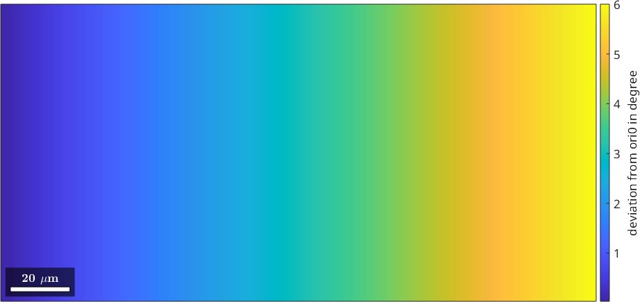

The colour changes smoothly from left to right because gradDir is xvector. With the default unit step, each column adds 0.03° about yvector. The first column is already one increment from ori0 because the default map coordinates start at one.

Further gradients can be superposed by changing axS, gradDir, or mori_angle and calling addFeature_simpleGradient again. In contrast, addFeature_circularSubgrain applies mori_angle as one total rotation. It changes the orientations inside a circular domain. Assign an existing map to eS.EBSDsim to start from measured or separately generated data.