Vector-valued spherical functions

A vector-valued spherical function collects several scalar functions on the sphere in one MATLAB array,

\[ f\colon \mathrm{S}^2\to\mathbb{R}^n. \]

Its output components are numerical values. This differs from a spherical vector field, whose output is a geometric vector, and from a spherical axis field, whose output is unchanged when its representative is reversed. Use a vector-valued S2Fun when the components should support MATLAB array indexing, concatenation and reduction. Component shape is independent of point-group invariance. Use symmetric spherical functions when all components share one symmetry.

plottingConvention.default('y↑→x');

How component arrays are laid out

MTEX always interprets the evaluation nodes as a column. The node index is the first dimension of the returned values. The dimensions of the spherical-function array begin with the second dimension.

For example, suppose four nodes \(v_1,\ldots,v_4\) are evaluated by six scalar functions stored as a \(3\times2\) spherical-function array. The returned array F has size \(4\times3\times2\), with

\[ F(i,:,1)=[f_1(v_i),f_2(v_i),f_3(v_i)] \]

and

\[ F(i,:,2)=[f_4(v_i),f_5(v_i),f_6(v_i)]. \]

fourNodes = [xvector;yvector;zvector; ...
  vector3d.byPolar(60*degree,45*degree)];
sixValueFunction = @(v) reshape([v.x,v.y,v.z,v.x.^2,v.y.^2,v.z.^2], ...
  length(v),3,2);
F = sixValueFunction(fourNodes);
valueArraySize = size(F);

Accordingly, valueArraySize is [4 3 2]. Index F(i,j,k) is the value at node i of component (j,k). This rule lets one evaluation retain both the node layout and the component-array layout.

Interpolate sampled component values

The same convention applies when fitting a harmonic representation. Here the two columns of sampleValues define two scalar functions at every node.

nodes = equispacedS2Grid('points',800);
nodes = nodes(:);
sampleValues = [S2Fun.smiley(nodes),nodes.x.*nodes.y];

interpolate places the two component dimensions after its hidden coefficient dimension. The resulting sF1 has size \(2\times1\).

sF1 = S2FunHarmonic.interpolate(nodes,sampleValues,'bandwidth',12, ...
  'weights','equal');
componentArraySize = size(sF1);

Plot the components

The scalar plotting commands also accept a vector-valued function. MTEX draws one panel per component rather than combining their values.

plot(sF1,'upper');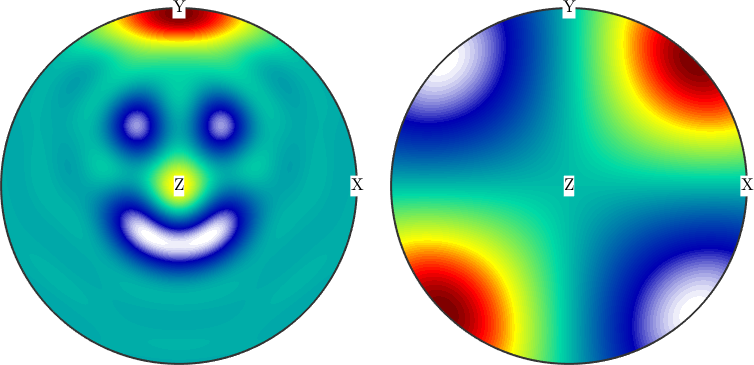

The first panel contains the smiley. The second has four lobes because the sign of \(xy\) alternates between neighboring quadrants. Separate panels are essential here: the two values are components, not the coordinates of arrows.

Construct from a function handle

A handle must return one row per input direction and one column per component. This example retains the original peaked scalar component and appends the Cartesian coordinate functions \(x\), \(y\) and \(z\).

fourComponentFunction = @(v) [exp(v.x+v.y+v.z) + ...
  50*(v.y-cos(pi/3)).^3.*(v.y-cos(pi/3)>0),v.x,v.y,v.z];

Passing the handle to the constructor applies quadrature. The harmonic cutoff is degree 50, and the resulting sF2 has size \(4\times1\).

sF2 = S2FunHarmonic(fourComponentFunction,'bandwidth',50);
handleArraySize = size(sF2);

Construct from harmonic coefficients

If the coefficients are already known, pass them directly to the S2FunHarmonic constructor. The first dimension of fhat is reserved for the coefficients of one scalar function. Component-array dimensions begin with its second dimension.

Thus, if \(\widehat f_1,\ldots,\widehat f_6\) are coefficient columns for the \(3\times2\) example above, their internal arrangement is

\[ \widehat F(:,:,1)=[\widehat f_1,\widehat f_2,\widehat f_3] \]

and

\[ \widehat F(:,:,2)=[\widehat f_4,\widehat f_5,\widehat f_6]. \]

sF3 = S2FunHarmonic(eye(9));

Each column of the identity selects one coefficient. Consequently, sF3 stores the first nine spherical harmonics as nine component functions. Most applications construct functions from values and never need to access this coefficient layout directly.

Index, concatenate and reshape components

Component arrays follow ordinary MATLAB indexing. Vertical concatenation combines the two functions in sF1 with the four in sF2, while indexing selects components.

sF4 = [sF1;sF2];
selectedFunctions = sF4(2:3);

Conjugation acts on the coefficients. Transpose and conjugate transpose rearrange the component dimensions in the usual MATLAB way.

conjugatedFunctions = conj(sF1);
transposedFunctions = sF1.';
conjugateTransposedFunctions = sF1';

length and size inspect the component array rather than the hidden coefficient dimension. Reshaping the nine functions in sF3 produces a \(3\times3\) spherical-function array.

numberOfFunctions = length(sF1);
shapeOfHandleFunctions = size(sF2);
sF3 = reshape(sF3,3,[]);

Integrate or reduce components

With no dimension argument, sum integrates every component over the sphere and mean returns the spherical mean of every component. Their outputs are numerical arrays with size(sF).

componentIntegrals = sum(sF1);
componentMeans = mean(sF1);

With a dimension argument, the same commands perform pointwise array reductions and return another spherical function.

rowSums = sum(sF3,2);
columnMeans = mean(sF3,1);

Pointwise minima and maxima

For a vector-valued function, pass an empty second argument and the component dimension as the third argument. The result is the pointwise minimum or maximum along that component dimension.

columnMinima = min(sF3,[],1);

A note on products

An older implementation note states that the matrix product is implemented per element and not as the usual matrix product. In the current implementation, a product between two S2FunHarmonic arrays is not implemented. Use .* for pointwise multiplication. Multiplication by a compatible numerical matrix uses the overloaded * operator.

close all

References

Next

Continue with Spherical kernel functions to construct radially symmetric building blocks for spherical functions.