S2VectorField handles three-dimensional functions on the sphere. For instance the gradient of an univariate S2FunHarmonic can return a S2VectorFieldHarmonic.
Defining a S2VectorFieldHarmonic
Definition via function values
At first we need some example vertices
nodes = equispacedS2Grid('points', 1e5);
nodes = nodes(:);
Next, we define function values for the vertices
y = vector3d.byPolar(sin(3*nodes.theta), nodes.rho+pi/2);Now the actual command to get sVF1 of type S2VectorFieldHarmonic
sVF1 = S2VectorFieldHarmonic.interpolate(nodes, y)sVF1 = S2VectorFieldHarmonic
bandwidth: 224Definition via function handle
If we have a function handle for the function we could create a S2VectorFieldHarmonic via quadrature. At first lets define a function handle which takes vector3d as an argument and returns again vector3d:
f = @(v) vector3d(v.x, v.y, 0*v.x);Now we can call the quadrature command to get sVF2 of type S2VectorFieldHarmonic
sVF2 = S2VectorFieldHarmonic(@(v) f(v))
% sVF2 = S2VectorFieldHarmonic.quadrature(@(v) f(v))
sVF2 = S2VectorFieldHarmonic
bandwidth: 128
Definition via S2FunHarmonic
If we directly call the constructor with a vector valued S2FunHarmonic with two or three entries it will create a S2VectorFieldHarmonic with sF(1) the polar angle and sF(2) the azimuth or sF(1), sF(2), and sF(3) the \(x\), \(y\), and \(z\) component.
sF = S2FunHarmonic(rand(10, 2));
sVF3 = S2VectorFieldHarmonic(sF)

sF = S2FunHarmonic(rand(10, 3));
sVF4 = S2VectorFieldHarmonic(sF)
sVF3 = S2VectorFieldHarmonic
bandwidth: 3
sVF4 = S2VectorFieldHarmonic
bandwidth: 3Operations
Basic arithmetic operations
Again the basic mathematical operations are supported:
addition/subtraction of a vector field and a vector or addition/subtraction of two vector fields
sVF1+sVF2; sVF1+vector3d(1, 0, 0);
sVF1-sVF2; sVF2-vector3d(sqrt(2)/2, sqrt(2)/2, 0);
multiplication/division by a scalar or a S2Fun
2.*sVF1; sVF1./4;
S2Fun.smiley .* sVF1;
dot product with a vector or another vector field
dot(sVF1, sVF2); dot(sVF1, vector3d(0, 0, 1));cross product with a vector or another vector field
cross(sVF1, sVF2); cross(sVF1, vector3d(0, 0, 1));mean vector of the vector field
mean(sVF1);rotation of the vector field
r = rotation.byEuler( [pi/4 0 0]);
rotate(sVF1, r);
pointwise norm of the vectors
norm(sVF1);Visualization
One can use the default plot-command
plot(sVF1);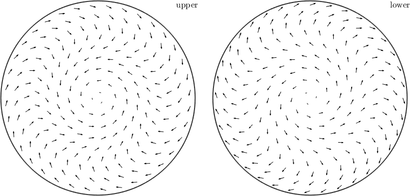
- same as quiver(sVF1)
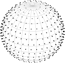
or the 3D plot of a sphere with the vectors on itself
clf;
quiver3(sVF2);