Spin Tensors as Infinitesimal Changes of Rotations

A spin tensor is a skew-symmetric matrix that describes an infinitesimal rotation. Its three independent entries give an axis scaled by an angle, or by an angular rate when the independent variable is time.

This page assumes the active rotations introduced in Defining Rotations, the multiplication order in Calculating with Rotations, and the tangent vectors introduced in Tangent Spaces.

MTEX uses a spinTensor as the matrix form of a tangent vector on the rotation group SO(3). MTEX calls its two coordinate representations left and right.

plottingConvention.default('y↑→x');

A Small Rotation

Start from a reference rotation and perturb it on the right about the Cartesian direction \((1,2,3)\). The constructor normalizes the axis, and the small angle is \(\delta=0.01^\circ\).

rotRef = rotation.byEuler(10*degree,20*degree,30*degree,'Bunge');
axis123 = vector3d(1,2,3);
delta = 0.01*degree;
increment = rotation.byAxisAngle(axis123,delta);
rotNext = rotRef * increment;

For the path \(R(\delta)=R\,P(\delta)\), a finite-difference approximation to the tangent matrix is

\[ T = \left.\frac{\mathrm d R(\delta)}{\mathrm d\delta}\right|_{0} \simeq \frac{R(\delta)-R}{\delta}. \]

T = (rotNext.matrix-rotRef.matrix) ./ delta

T =
   -0.5399   -0.6025    0.5816
    0.7530   -0.5816    0.1368
   -0.2648    0.1140    0.0122

The tangent matrix T is not itself skew symmetric. Dividing out the reference rotation from the right or left gives two skew representations of the same tangent:

\[ S_{\rm left}=T R^{-1}, \qquad S_{\rm right}=R^{-1}T. \]

invR = matrix(inv(rotRef));
SLeft = T * invR
SRight = invR * T

SLeft =
   -0.0001   -0.9575    0.2758
    0.9575   -0.0001    0.0850
   -0.2758   -0.0850   -0.0000
SRight =
   -0.0001   -0.8018    0.5345
    0.8018   -0.0001   -0.2672
   -0.5345    0.2673   -0.0000

The small diagonal entries are a second-order finite-difference residual. Constructing a spinTensor extracts the antisymmetric part. Its axial vector uses the convention

\[ S\,x = \omega \mathbin{\times} x. \]

Multiplication by \(\sqrt{14}\) undoes the normalization of \((1,2,3)\). The right coordinates recover the input axis, while the left coordinates are that axis expressed after the reference rotation.

scaledAxisRight = vector3d(spinTensor(SRight)) * sqrt(14)
scaledAxisLeft = vector3d(spinTensor(SLeft)) * sqrt(14)

scaledAxisRight = vector3d (y↑→x)
  x y z
  1 2 3
 
scaledAxisLeft = vector3d (y↑→x)
       x      y      z
  -0.318   1.03   3.58

Seeing the Instantaneous Motion

A spin tensor is easier to read through its action on a direction. The red arrow is the rotation axis, and the grey arrow is a direction on the black orbit. The blue arrow is its instantaneous velocity.

rotationAxis = normalize(axis123);
v0 = rotation.byAxisAngle(rotationAxis,pi/2) * ...
  normalize(vector3d(1,-2,1));
t = linspace(0,2*pi,300);
orbit = rotation.byAxisAngle(rotationAxis,t) * v0;
velocity = cross(rotationAxis,v0);

plot3(orbit.x,orbit.y,orbit.z,'k','linewidth',1.5)
hold on
arrow3d(1.25*rotationAxis,'faceColor','red')
arrow3d(0.999*v0,'faceColor',[.45 .45 .45])
arrow3d(0.9*normalize(velocity),'anchor',v0,'faceColor','blue',...
  'arrowWidth',0.035)
hold off
axis equal off

% look at the orbit plane from above, so the three arrows do not overlap
view(-180,25)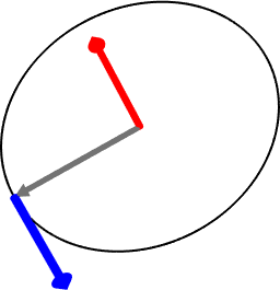

Notice that the blue arrow is tangent to the black orbit. It is also perpendicular to both the red axis and the grey direction, as the cross product in \(Sx=\omega\mathbin{\times}x\) requires.

When a Spin Tensor Is a Rate

The matrices above are derivatives with respect to rotation angle, not time. They become angular-velocity tensors only for a time-dependent rotation \(R(t)\):

\[ W_{\rm left}=\dot R R^{-1}, \qquad W_{\rm right}=R^{-1}\dot R. \]

In continuum mechanics the spatial velocity gradient \(L=\nabla v\) splits into a symmetric rate of deformation and a spin tensor,

\[ L=D+W, \qquad D=\tfrac12(L+L^T), \qquad W=\tfrac12(L-L^T). \]

Thus spinTensor can store either a finite rotation increment or a rate. Its units and physical meaning come from the quantity used to construct it.

Finite Changes with Log and Exp

Matrix subtraction is useful only for a small perturbation. For a finite change, log returns the exact tangent generator at a reference rotation. Here the perturbation angle is one radian.

finiteAngle = 1;
finiteIncrement = rotation.byAxisAngle(axis123,finiteAngle);
rotEnd = rotRef * finiteIncrement;

SRight = log(rotEnd,rotRef,SO3TangentSpace.rightSpinTensor)
SLeft = log(rotEnd,rotRef,SO3TangentSpace.leftSpinTensor)

SRight = spinTensor (y↑→x)
  rank: 2 (3 × 3)
 
 *10^-2
      0 -80.18  53.45
  80.18      0 -26.73
 -53.45  26.73      0
 
SLeft = spinTensor (y↑→x)
  rank: 2 (3 × 3)
 
 *10^-2
      0 -95.75  27.58
  95.75      0    8.5
 -27.58   -8.5      0

Unlike the finite-difference matrices, the displayed results are exactly skew symmetric. Their axial vectors point along the right and left coordinate triplets shown above, with length equal to the one-radian angle.

The vector forms contain the same three components without the skew-symmetric matrix wrapper.

vRight = log(rotEnd,rotRef,SO3TangentSpace.rightVector);
vLeft = log(rotEnd,rotRef,SO3TangentSpace.leftVector);

spinVectorResidual = [norm(vector3d(SRight)-vector3d(vRight)),...
  norm(vector3d(SLeft)-vector3d(vLeft))]

spinVectorResidual =
     0     0

Both zero residuals confirm that spin tensors and rotation vectors are two representations of the same tangent coordinates.

exp and the spinTensor form of exp apply those coordinates back at the reference rotation. All four reconstructions below should return rotEnd.

rotFromRightVector = exp(vector3d(vRight),rotRef,...
  SO3TangentSpace.rightVector);
rotFromLeftVector = exp(vector3d(vLeft),rotRef,...
  SO3TangentSpace.leftVector);
rotFromRightSpin = exp(SRight,rotRef,...
  SO3TangentSpace.rightSpinTensor);
rotFromLeftSpin = exp(SLeft,rotRef,...
  SO3TangentSpace.leftSpinTensor);

roundTripError = angle(rotEnd,[rotFromRightVector,rotFromLeftVector,...
  rotFromRightSpin,rotFromLeftSpin]) ./ degree

roundTripError =
   1.0e-05 *
         0    0.1708         0    0.1708

The displayed errors are at floating-point level. Rotation logarithms use a principal branch with angles up to \(180^\circ\). At exactly \(180^\circ\) the two signs of the axis describe the same rotation, so the logarithm is not unique.

Under Crystal Symmetry

For an orientation, right coordinates belong to the crystal frame and left coordinates belong to the specimen frame. The crystal frame is the Cartesian reference frame glued to the phase's lattice basis. The specimen frame is the reference frame in which the sample is expressed.

Define a one-radian perturbation about the trigonal crystal direction \((1,2,\bar3,3)\) and apply it on the right.

cs = crystalSymmetry('321');
oriRef = orientation.byEuler(10*degree,20*degree,30*degree,'Bunge',cs);
crystalIncrement = orientation.byAxisAngle(Miller(1,2,-3,3,cs),1);
oriEnd = oriRef * crystalIncrement;

The right tangent is expressed in crystal coordinates. Converting it to Miller indices recovers the direction used above.

crystalAxis = Miller(log(oriEnd,oriRef,...
  SO3TangentSpace.rightVector),oriEnd.CS);
recoveredCrystalAxis = round(crystalAxis)

recoveredCrystalAxis = Miller (321)
  h  k  i  l
  1  2 -3  3

The left tangent gives the same change in specimen coordinates.

specimenVector = log(oriEnd,oriRef,SO3TangentSpace.leftVector)

specimenVector = SO3TangentVector (y↑→x)
 intern symmetries: 321 → y↑→x
 tangentSpace: leftVector
      x     y     z
  0.162 0.428 0.889

Applying the crystal-frame tangent returns the endpoint. The displayed value is the angular round-trip error in degrees.

oriFromCrystalVector = exp(crystalAxis,oriRef,...
  SO3TangentSpace.rightVector);
orientationRoundTripError = angle(oriEnd,oriFromCrystalVector) ./ degree

orientationRoundTripError =
     0

orientation.log first chooses the shortest symmetry-equivalent change. This makes the tangent describe the two crystal orientations rather than their stored representatives. Pass 'noSymmetry' only when the unreduced rotation representatives are the intended objects.

The Maths Behind Left and Right Coordinates

Let \([\omega]_\times\) denote the skew matrix whose axial vector is \(\omega\). For the right-perturbed path \(R(\delta)=R\exp(\delta[\omega]_{\times})\),

\[ T=R[\omega]_{\times}, \qquad S_{\rm right}=[\omega]_{\times}, \qquad S_{\rm left}=R[\omega]_{\times}R^{-1}. \]

Conjugating a skew matrix rotates its axial vector. Therefore \(\omega_{\rm left}=R\omega_{\rm right}\). Left and right describe one tangent at one base rotation; only the coordinate frame changes.

References

Next

Tensors introduces the typed tensors used in the material description, including velocityGradientTensor. Taylor Model computes crystallographic spin, and Texture Evolution applies those increments to a population of crystal orientations.

References

- A. Morawiec, Orientations and Rotations: Computations in Crystallographic Textures, Springer, 2004, develops the geometry of rotation space and small orientation changes.
- A. Morawiec, The rotation rate field and geometry of orientation space, Journal of Applied Crystallography 23 (1990) 374--377, relates infinitesimal rotations to texture evolution.
- M. E. Gurtin, E. Fried, and L. Anand, The Mechanics and Thermodynamics of Continua, Cambridge University Press, 2010, develops stretching and spin in continuum kinematics.