While the linear elastic model for anisotropic materials is based on the fourth order elastic stiffness tensor C the linear elastic model for isotropic models is most often developed in terms of the elastic moduli shear, bulk, Youngs modulus and the Poisson ratio.
The single crystal stiffness tensor
Lets start our discussion with a single crystal stiffness tensor of Albite.
% density (g/cm3)
 rho= 2.6230;
%
% crystal symmetry & frame
cs = crystalSymmetry('-1', [8.290 12.966 7.151], [91.18 116.31 90.14]*degree,...
  'x||a*','y||b', 'mineral','An0 Albite 2016');

% the stiffness tensor C in (GPa)
C = stiffnessTensor(...
  [[  68.30   32.20   30.40    4.90   -2.30  -0.90];...
  [   32.20  184.30    5.00   -4.40   -7.70  -6.40];...
  [   30.40    5.00  180.00   -9.20    7.50  -9.40];...
  [    4.90   -4.40   -9.20   25.00   -2.40  -7.20];...
  [   -2.30   -7.70    7.50   -2.40   26.90   0.60];...
  [   -0.90   -6.40   -9.40   -7.20    0.60  33.60]],...
  cs,'density',rho)
C = stiffnessTensor (An0 Albite 2016)
density: 2.623
unit : GPa
rank : 4 (3 x 3 x 3 x 3)
tensor in Voigt matrix representation:
68.3 32.2 30.4 4.9 -2.3 -0.9
32.2 184.3 5 -4.4 -7.7 -6.4
30.4 5 180 -9.2 7.5 -9.4
4.9 -4.4 -9.2 25 -2.4 -7.2
-2.3 -7.7 7.5 -2.4 26.9 0.6
-0.9 -6.4 -9.4 -7.2 0.6 33.6The effective isotropic stiffness tensor
An isotropic Albite material we assume here to consist of randomly oriented grains forming an uniform (isotropic) texture. In this case the Voigt and Reuss averages provide upper and lower bounds for the elastic properties of the material.
[C_iso_Voigt,C_iso_Reuss,C_iso_Hill] = mean(C,uniformODF(C.CS))C_iso_Voigt = stiffnessTensor (y↑→x)
density: 2.623
unit : GPa
rank : 4 (3 x 3 x 3 x 3)
tensor in Voigt matrix representation:
118.33 35.47 35.47 0 0 0
35.47 118.33 35.47 0 0 0
35.47 35.47 118.33 0 0 0
0 0 0 41.43 0 0
0 0 0 0 41.43 0
0 0 0 0 0 41.43
C_iso_Reuss = stiffnessTensor (y↑→x)
density: 2.623
unit : GPa
rank : 4 (3 x 3 x 3 x 3)
tensor in Voigt matrix representation:
93.83 34.16 34.16 0 0 0
34.16 93.83 34.16 0 0 0
34.16 34.16 93.83 0 0 0
0 0 0 29.84 0 0
0 0 0 0 29.84 0
0 0 0 0 0 29.84
C_iso_Hill = stiffnessTensor (y↑→x)
density: 2.623
unit : GPa
rank : 4 (3 x 3 x 3 x 3)
tensor in Voigt matrix representation:
106.08 34.81 34.81 0 0 0
34.81 106.08 34.81 0 0 0
34.81 34.81 106.08 0 0 0
0 0 0 35.63 0 0
0 0 0 0 35.63 0
0 0 0 0 0 35.63The elastic moduli
The actual elastic properties of the material depend on the geometric microstructure and can not be computed without additional knowledge.
Based on the Voigt effective stiffness tensor we may now compute upper, directional independent bounds for all elastic moduli:
G = C_iso_Voigt.shearModulus
K = C_iso_Voigt.bulkModulus
E = C_iso_Voigt.YoungsModulus(xvector)
nu = C_iso_Voigt.PoissonRatio
G =
41.4333
K =
63.0889
E =
101.9759
nu =
0.2306From the elastic moduli to the elastic tensors
Furthermore, any two of them entirely describe the linear elastic behavior of the material. In particular, we may recover the isotropic stiffness tensor from the bulk and shear moduli alone:
% the matrix entries
C11 = K+(4/3)*G ; C12=C11-2*G; C44=(C11-C12)/2;

% this gives exactly the effective Voigt stiffness tensor as computed above
stiffnessTensor(...
  [[  C11     C12    C12    0.0     0.0    0.0];...
  [   C12     C11    C12    0.0     0.0    0.0];...
  [   C12     C12    C11    0.0     0.0    0.0];...
  [   0.0     0.0    0.0    C44     0.0    0.0];...
  [   0.0     0.0    0.0    0.0     C44    0.0];...
  [   0.0     0.0    0.0    0.0     0.0    C44]],cs)
ans = stiffnessTensor (An0 Albite 2016)
unit: GPa
rank: 4 (3 x 3 x 3 x 3)
tensor in Voigt matrix representation:
118.33 35.47 35.47 0 0 0
35.47 118.33 35.47 0 0 0
35.47 35.47 118.33 0 0 0
0 0 0 41.43 0 0
0 0 0 0 41.43 0
0 0 0 0 0 41.43or from the Youngs modulus and the Poisson ratio
S11 = (1/E); S12 = (-nu/E); S44 = 2*(S11-S12);

inv(complianceTensor(...
 [[  S11     S12    S12    0.0     0.0    0.0];...
 [   S12     S11    S12    0.0     0.0    0.0];...
 [   S12     S12    S11    0.0     0.0    0.0];...
 [   0.0     0.0    0.0    S44     0.0    0.0];...
 [   0.0     0.0    0.0    0.0     S44    0.0];...
 [   0.0     0.0    0.0    0.0     0.0    S44]],cs))
ans = stiffnessTensor (An0 Albite 2016)
unit: GPa
rank: 4 (3 x 3 x 3 x 3)
tensor in Voigt matrix representation:
118.33 35.47 35.47 0 0 0
35.47 118.33 35.47 0 0 0
35.47 35.47 118.33 0 0 0
0 0 0 41.43 0 0
0 0 0 0 41.43 0
0 0 0 0 0 41.43Formulas between the elastic moduli
As a consequence, Young's modulus and the Poisson ratio can be computed directly from the bulk and shear modulus (and vice versa)
% formulae for the Poisson ratio
(E/G-2)/2
(3*K-E)/(6*K)

% formulae for the Young's modulus
2*G*(1+nu)
3*K*(1-2*nu)
ans =
0.2306
ans =
0.2306
ans =
101.9759
ans =
101.9759Lame constants
The second way to represent the elastic behavior of an isotropic medium is by means of the Lame constants
lambda = nu/(1-2*nu) /(1+nu) * E;
mu = G;
In terms of the Lame constants the stiffness tensor is given by
2 * mu * stiffnessTensor.eye(cs) + lambda * dyad(tensor.eye,tensor.eye)ans = stiffnessTensor (An0 Albite 2016)
unit: GPa
rank: 4 (3 x 3 x 3 x 3)
tensor in Voigt matrix representation:
118.33 35.47 35.47 0 0 0
35.47 118.33 35.47 0 0 0
35.47 35.47 118.33 0 0 0
0 0 0 41.43 0 0
0 0 0 0 41.43 0
0 0 0 0 0 41.43and we may directly formulate Hooks law
eps = strainTensor.rand(cs);

sigma = C_iso_Voigt : eps
sigma = stressTensor (y↑→x)
rank: 2 (3 x 3)
77.13 19.11 31.25
19.11 75.83 39.35
31.25 39.35 65.83in terms of the Lame constants by
sigma = stressTensor(2 * mu * eps + lambda * trace(eps) * tensor.eye)sigma = stressTensor (An0 Albite 2016)
type: Lagrange
rank: 2 (3 x 3)
77.13 19.11 31.25
19.11 75.83 39.35
31.25 39.35 65.83Hashin Shtrikman Bounds
While the Voigt and Reuss bounds are tight without additional assumptions, the extreme cases require a very specific layered microstructure. If one additionally assumes that the material is quasihomogeneous, i.e., it is constant elastic properties within each subregion that is significantly larger then the grain size, then the Voigt and Reuss bounds are to wide. More narrow bounds for this settings have been established by Hashin and Shtrikman in 1962.
The following deviation follows the paper by J.M. Brown (2015) Determination of Hashin-Shtrikman bounds on the isotropic effective elastic moduli of polycrystals of any symmetry, Computers & Geosciences, 80 (2015) 95-99.
The upper and lower Hashin-Shtrikman bounds for the bulk and shear moduli are found as a solution of an optimization problem. Lets first set up the search domain
% define a 2 dimensional domain of bulk and shear moduli
KMin = 1; KMax = 150; % minimum and maximum bulk moduli
GMin = 1; GMax = 150; % minimum and maximum shear moduli
Ko = linspace(KMin,KMax,300);
Go = linspace(GMin,GMax,300);
[G0Mesh,K0Mesh] = meshgrid(Go,Ko);
Next the initial stiffness tensor is updated such that the residual stiffness tensor R remains either positive or negative definite.
[khs, ghs, def] = HashinShtrikmanModulus(C,K0Mesh,G0Mesh);

subplot(1,2,1)
imagesc(Go,Ko,khs)
set(gca,'YDir','normal')
title('khs')
xlabel('shear modulus')
ylabel('bulk modulus')
colorbar%('location','southoutside')
axis equal tight

subplot(1,2,2)
imagesc(Go,Ko,ghs)
set(gca,'YDir','normal')
xlabel('shear modulus')
ylabel('bulk modulus')
title('ghs')
colorbar%('location','southoutside')
axis equal tight

%subplot(1,3,3)
%imagesc(G0,K0,minmax)
%set(gca,'YDir','normal')
%title('minmax')
%colorbar('location','southoutside')
%xlabel('shear modulus')
%ylabel('bulk modulus')
%axis equal tight
Warning: Tensor is not positive definite
Warning: Tensor is not positive definite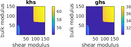
lower and upper Hashin Shtrikman bulk and shear modulus bounds
We find the lower Hashin Shtrikman bound of the bulk modulus by minimizing the effective Hashin Shtrikman bulk modulus over the positive definite domains of the residual stiffness tensor R. Accordingly we find the upper bound as the maximum over the negative definite domain.
khsLower = max(khs(def==1));
khsUpper = min(khs(def==-1));

ghsLower = max(ghs(def==1));
ghsUpper = min(ghs(def==-1));
Lower and upper bounds are marked in the plots below.
subplot(1,2,1)
hold on
[i,j] = find(khs == khsLower);
plot(Go(j),Ko(i),'o','MarkerEdgeColor','w','linewidth',2)
[i,j] = find(khs == khsUpper);
plot(Go(j),Ko(i),'o','MarkerEdgeColor','w','linewidth',2)
hold off

subplot(1,2,2)
hold on
[i,j] = find(ghs == ghsLower);
plot(Go(j),Ko(i),'o','MarkerEdgeColor','w','linewidth',2)
[i,j] = find(ghs == ghsUpper);
plot(Go(j),Ko(i),'o','MarkerEdgeColor','w','linewidth',2)
hold off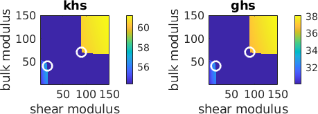
Comparison of the bounds
Finally we compare the upper and lower Hashin Shtrikman bounds with the Voigt and Reuss bounds.
KReuss = C_iso_Reuss.bulkModulus;
KHill = C_iso_Hill.bulkModulus;
GVoigt = C_iso_Voigt.shearModulus;
GReuss = C_iso_Reuss.shearModulus;
GHill = C_iso_Hill.shearModulus;

disp(' ')
disp('bulk modulus')
cprintf([K,khsUpper,KHill,khsLower,KReuss],...
  '-Lc',{'Voigt' '+HS' 'Hill' '-HS' 'Reus'})
disp(' ')
disp('shear modulus')
cprintf([GVoigt,ghsUpper,GHill,ghsLower,GReuss],...
  '-Lc',{'Voigt' '+HS' 'Hill' '-HS' 'Reus'})
disp(' ')
bulk modulus
Voigt +HS Hill -HS Reus
63.0889 60.326 58.5696 57.107 54.0503
shear modulus
Voigt +HS Hill -HS Reus
41.4333 36.7537 35.6344 32.8495 29.8355Note, that upper and lower bounds for all other elastic moduli can be computed from these upper and lower bounds of the bulk and shear modulus.